Inversion Recovery Experiments in OVJ
The longitudinal relaxation time T1 can be determined from an inversion-recovery experiment. This is another good example to demonstrate the arrying capabilities in OVJ. If you haven’t read the section about how to array parameters in OVJ, we would suggest doing this first before you start to follow this example.
The following pre-requisites are assumed:
- A sample is inserted in the probe.
- The 90 degree pulse length is know. To determine the correct pulse length please follow the steps outlined in the section Calibrating a 90º Pulse.
Acquire the Inversion Recovery Data
To perform the inversion-recovery experiment follow these steps:
-
Select the PROTON experiment (
seqfile='s2pul'). -
Enter the pulse for the 90 degree pulse (pw) and the 180 degree inversion pulse (d1).
-
Enter a value for d1. This is the repetition time of the experiment and it should typically be set to a value of 5 times the T1 relaxation time of the nucleus. For example, if the relaxation time of the water protons is about 1 s, the value for d1 should be set to 5 s. This ratio can be reduced to speed up the experiment, however, if the repetition time is too short, the measured value for T1 will be incorrect.
-
For the inversion-recovery experiment we will array the d2 parameter
1array('d2',30,0.05,0.05) -
Press ‘Go’ to start the acquisition or type
goand press enter in the OVJ command line. -
Once the aquisition is finished save the data.
Determining T1 in OVJ
To determine T1 in OVJ follow these steps:
-
Select the last spectrum of the array using the
dscommand. Here, we use spectrum number 15. Alternatively, you can select any spectrum with sufficient signal-to-noise.1ds(15) -
Phase the spectrum using the autophase function
aph:1aphOnce all spectra are phased, you can display all spectra horizontally using the
dsshcommand:1dsshThe result should like like the example below
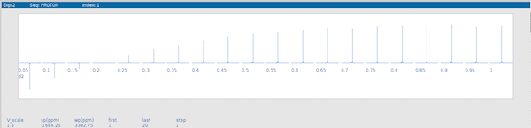
If the spectra look like the data shown in the image proceed to the next step.
-
Select the last spectrum using the
ds(15)command. -
Next, we need to set a threshold for the peak picking algorithm. The threshold is set using the
thparameter. In this example, we will set a threshold of 10.1th=10You can also use the horizontal line marker to adjust a threshold. Set the threshold to a value that only one peak is above the threshold.
-
In the next step the peak amplitudes for each spectrum are determined using the
dllandfp(find peak) command. Only peaks are considered that are above the threshold value.1 2dll fp -
To get the T1 relaxation time, the t1 OVJ macro can be used. To run the macro, enter t1 in the OVJ command line and press enter.
1t1 -
Display the fitting results using these OVJ command line commands:
1 2center explYou should see a result similar to the one shown below.

The fit values returned by the t1 macro can be seen in the Process tab under Text output.

The t1 macro will create an output file located in the current experiment folder. The path the folder is (N corresponds to the experiment number). The number of the current experiment can be seen in the top left part of the display tab or using the curexp? command in the OVJ command line.
|
|
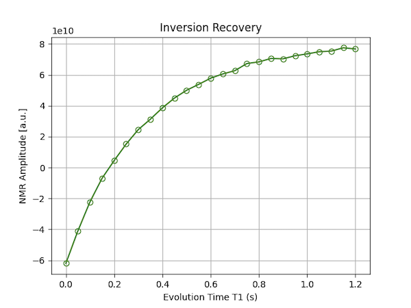
Evaluation with dnplab
The inversion-recovery experiment can also be analyzed using DNPLab. First, make sure DNPLab is installed:
|
|
A typical processing script is given below:
|
|
The first subfigure can be used to determine the noise and signal region. The second figure shows the T1 recovery curve. An example for the second figure is shown below.