Calibrating the 90º Pulse Length
Calibrating the 90º pulse length is a good example for arraying parameters in OVJ. If you haven’t read the section about how to array parameters in OVJ, we would suggest doing this first before you start to follow this example.
To calibrate the 90 degree pulse length follow these steps:
- Insert a water sample into the probe.
- Select the PROTON sequence in OVJ.
- Set the following parameters in OVJ.
- Set the sweep width (
sw) to a value that the NMR signal (here a single peak from the water sample) is fully within the sweep width of the experiment and some noise is shown left and right to the peak. - Set the number of scans (
nt) to a value to obtain a clear signal (not too noisy). - Set the number of acquired points
npto 4096, to acquire 2048 complex points.
- Set the sweep width (
- Array the parameter
pwfrom 0 to about three times the expected pulse length for the 90 degree pulse. In this example we set the array the parameter from 0 to 15 µs with a step size of 0.25 µs. - Start the acquisition of the experiment and save the data once the experiment has finished.
The obtained data can be either analyzed in OVJ or dnplab to determine the length of the 90 degree pulse.
Determining the 90 Degree Pulse Length in OVJ
To process the nutation experiment in OVJ follow these steps:
-
After the acquisition select the ‘Process’ tab
- Select Display and set the display mode for the spectrum to ‘Phased’
- Select a spectrum that with sufficient signal-to-noise and phase the spectrum. Use a spectrum with a shorter pulse length, don’t use the last spectrum of the nutation experiment. The same phase correction is applied to all spectra in the array.
-
If the sweep width of the spectrum is large, zoom into the region with the peak.
- Move the mouse cursor to the left of the peak and press the left mouse button. Next, move the mouse cursor to the right of the peak and click the right mouse button. The selected region is shown between the two red lines.
- Click on the zoom button in the toolbar to the left to zoom into the region defined by the two red lines.

-
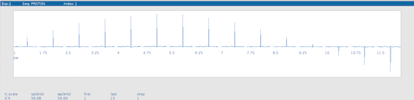
To show all spectra horizontally aligned, together with their respective pulse length
- Press the |||| button to show all spectra next to each other

- Next, click # to cycle through the acquisition number or the array parameter

-
To show all spectra of the array press the # button in the toolbar
-
The spectrum with the largest peak corresponds to the 90 degree pulse width. In this example the optimum pulse length is 4.75 µs.
Determining the 90 Degree Pulse Length in DNPlab
The nutation experiment can also be analyzed in DNPLab. If you haven’t installed DNPLab, this can be easily done using pip:
|
|
A typical DNPLab script to determine the 90 degree pulse length is given below:
|
|
This processing script first will load the data and does a Fourier transformation of the FID. Next, a DC offset will be removed using the remove_background function. Next, the NMR peak intensity is integrated using the integrate function and the data is plotted using the fancy_plot function.
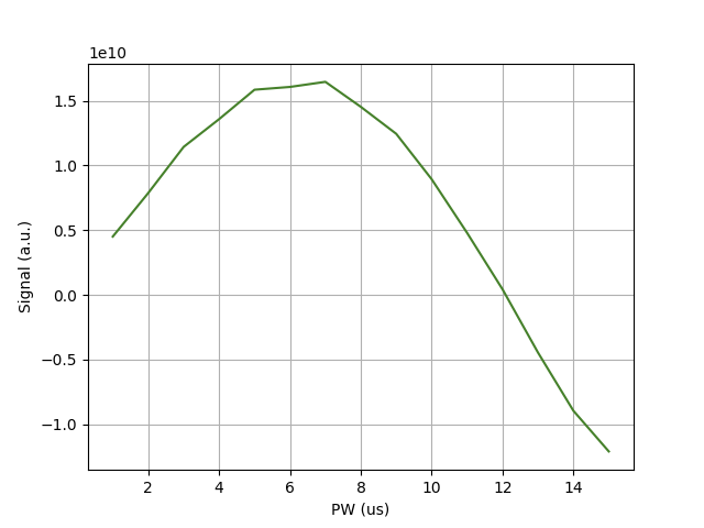
In the example the 90 degree pulse length is about 2.35 µs, and the 180 degree pulse length is about 4.7 µs.
Note
Different probes will have different pulse lengths for the 90 degree pulse. The pulse length also depends on the RF power. Higher RF power will result in a short pulse length. However, you should not exceed the maximum pulse power specified by the manufacturer to avoid damaging the probe.