This is the multi-page printable view of this section. Click here to print.
Software
- 1: Open VnmrJ
- 1.1: Overview
- 1.2: System Installation
- 1.2.1: Installing Open VnmrJ (Bridge12 Version)
- 1.2.1.1: Installing OVJ-B12
- 1.2.2: Setting Up the Hardware
- 1.2.2.1: Connecting the NMR Probe
- 1.2.2.2: Connecting an External Amplifier
- 1.2.2.3: External Trigger
- 1.3: Getting Started
- 1.3.1: Launching OVJ
- 1.3.2: Tuning the Probe
- 1.3.2.1: Using the nanoVNA
- 1.3.3: Acquiring a Proton Spectrum
- 1.3.3.1: Processing 1D Spectra in DNPLab
- 1.3.4: Saving the NMR Spectrum
- 1.4: Advanced Experiments
- 1.4.1: Arraying Parameters
- 1.4.2: Calibrating the 90º Pulse Length
- 1.4.3: Inversion Recovery Experiments in OVJ
- 1.4.4: Creating a Study in OVJ
- 1.5: DNP Experiments using OVJ
- 1.5.1: Controlling the MPS from OVJ
- 1.5.2: 1H ODNP Spectroscopy
- 1.5.3: DNP Power Build-UP (Saturation) Cruve
- 1.5.4: Using the External MPS Trigger
- 1.6: Reference
- 1.6.1: OVJ Commands
- 1.6.2: Pulse Programming
- 1.6.2.1: Pulse Elements
- 1.6.2.2: Phase Cycling
- 1.6.2.3: Pulse Sequence Parameters
- 1.6.2.4: ACODE
- 1.6.2.5: Hardware Control
- 1.6.3: OVJ Manuals
- 1.7: Frequently Asked Questions
- 2: SpecMan4EPR
- 2.1: Overview
- 2.2: Installation
- 2.3: Configuration
- 2.4: Magnet Control
- 2.4.1: Superconducting Magnets
- 2.4.1.1: SpecMan Magnet Control GUI
- 2.4.1.2: Heater Control
- 2.4.1.3: Operating the Magnet
- 2.5: Troubleshooting
- 2.5.1: SpecMan4EPR
- 2.5.2: Magnet
- 3: System Monitor - pyB12Logger
- 4: DNPLab
1 - Open VnmrJ

Welcome to the online documentation of Open VnmrJ for the Bridge12 Single Channel NMR (SCN) spectrometer. Open VnmrJ is an open-source software package designed for the acquisition, analysis, and processing of NMR data.
Bridge12 uses Open VnmrJ to control the Bridge12 SCN spectrometer. For Overhauser-DNP enhanced NMR spectroscopy, the Bridge12 Microwave Power Source (MPS) can also be controlled through OVJ.
The documentation provided here covers basic experiments, mainly focusing on the acquisition of Overhauser-DNP enhanced 1H NMR spectra.
For an in-depth documentation of OVJ please visit the Open VnmrJ website or consult the pdf documentation installed with the software.
1.1 - Overview
Open VnmrJ (OVJ)
Open VnmrJ (OVJ) is an open-source software package designed for the acquisition, analysis, and processing of nuclear magnetic resonance (NMR) spectral data. It is an extension of the popular VnmrJ software, which was originally developed by Varian (later Agilent) for NMR data processing and acquisition. OVJ provides a flexible and customizable platform for researchers to acquire, perform advanced data analysis, and visualize NMR experiments.
OVJ offers a wide range of features and tools to facilitate NMR data processing. It includes functionalities for Fourier transformation, baseline correction, peak picking, spectral fitting, and data manipulation. OVJ supports various 1D or multi-dimensional NMR experiment types, for solution- and solid-state NMR spectroscopy.
OVJ is entirely open source. The software’s source code is freely available and can be modified and customized by the user community. This allows researchers to adapt the software to their specific needs, add new functionalities, or contribute to the development and improvement of the software itself.
The software provides a user-friendly interface, making it easily accessible to both novice and experienced users. It offers a range of visualization tools, such as 1D and 2D spectral displays, contour plots, and integration windows, to aid in data interpretation. Additionally, the software supports automation and scripting capabilities, enabling users to streamline their workflows and automate repetitive tasks.
OVJ Resources
- Further information is available on the Open VnmrJ webpage.
- To contribute to the project check out the How to join this project webpage for more information.
- The source code for OVJ is hosted on GitHub.
- Please report issues on the Issues Page of the GitHub Repository
Bridge12 Version of Open VnmrJ

Bridge12 uses a customized version of OVJ to control:
- The Bridge12 Single Channel NMR (SCN) spectrometer
- The Bridge12 Shim Power Supply (Bridge12 SPS)
- The Bridge12 Microwave Power Source (MPS) for Overhauser-DNP spectroscopy.
All functionality of OVJ is available in the Bridge12 version of OVJ, but new functionality is added to communicate with the Bridge12 instruments.
Syntax Highlighting
Syntax highlighting is used throughout this documentation. Below are some examples for reference:
Shell Command
|
|
Python Script
|
|
1.2 - System Installation
1.2.1 - Installing Open VnmrJ (Bridge12 Version)
The following pages provide a step-by-step guide how to install the Bridge12 version of OVJ and getting the computer ready for your first NMR experiment.
System Requirements
The following computer hardware will be required:
| Parameter | Requirement |
|---|---|
| Computer | 64-bit System |
| Free Disk Space | > 4 GB |
| Operating System | Ubuntu 20.04 LTS system |
| Python | Python (> 3.8) pyserial (version 3.5) |
This installation guide assumes that you are installing OVJ_B12 on a clean installation of Ubuntu 20.04 LTS. To install OVJ, please create an user account called vnmr1 during the installation process. This should be an account with administrator rights.
Once the Ubuntu installation is finished, please log in as this user.
1.2.1.1 - Installing OVJ-B12
Note
Open VnmrJ is automatically installed when installing OVJ-B12, the Bridge12 version of OVJ. OVJ does not have to be installed separately.
Bridge12 does not offer a pre-compiled version of OVJ-B12. Instead, the package has to be build on the computer that is used to operate the spectrometer. However, the installation process is streamlined and does not require any specific programming skills besides navigating through some terminal windows.
Preparing the System
-
Start by opening a terminal window and update all installed packages to the latest version:
1
2
sudo apt-get update sudo apt upgradeThe best way to install OVJ-B12 is by using the GitHub repository. Updates are pushed to the GitHub repository and can be installed by the user from there.
-
Install git and python3-pip
1
2
sudo apt install python3-pip sudo apt install gitTo communicate with the NMR spectrometer and the Bridge12 MPS a serial connection to the periphery is required. OVJ-B12 uses Python and the pyserial Python package for this purpose, which can be installed through pip.
1sudo pip3 install pyserial==3.5
Cloning the Repository
-
To clone the GitHub repository, open a terminal window
1git clone git@github.com:Bridge12Technologies/OpenVnmrJ_B12TOnce the repository is downloaded change into the directory …..
Building the OVJ-B12 Package
-
Build the package. As a first step in the installation, the OpenVnmrJ and ovjTools repositories will be automatically downloaded. The complete build processes takes about 10 minutes.
1sudo ./buildb12We recommend opening a new console tab in the terminal window to monitor the build process. To do this copy and paste the command (tail -f) with the corresponding file shown in the console after starting the build process into the new console tab of the terminal window.

-
Once the build is finished check the build process with
1./whatsinThe output should report 0 Errors and 0 Build Terminations for a successful build.
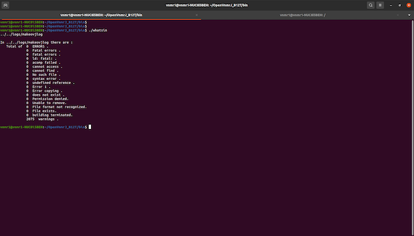
If the build succeeded the folder ~/ovjbuild/dvdimageB12 is created.
Install OVJ-B12
-
To install OVJ-B12 change to the dvdimageB12 directory and execute ./load.nmr
1
2
cd ~/ovjbuild/dvdimageB12 ./load.nmrA popup window will appear, press install to continue with the installation.

-
When asked to update users start the vnmrjAdmin program located on the Desktop. The program should start automatically. In vnmrjAdmin go to Configure -> Users -> Update users …
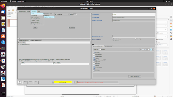
and add all users (vnmr1, service and walkup if they were created) to the right side. Then press “update users”

Once all users are updated, the bottom status line in OpenVnmrJAdmin will show “Update User Completed All Requested Users”. Once you see this message, close OpenVnmrJAdmin.
-
After this, the system will open a new terminal window and the user has to answer a few questions. Please answer both questions with y(yes).
1
2
Standard configurations include the walkup and service accounts. Would you like to make them now? (y/n)1 2Shall this system be configured as a spectrometer (see image below). Would you like to configure it now? (y/n)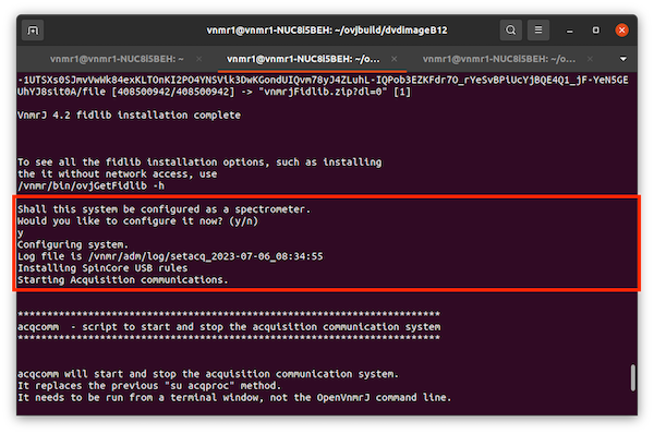
-
Installing NMRPipe is optional and can be answered with n(no).
-
We recommend to install the OVJ manuals. When asked to install the manuals please answer the question with y(yes).

Finish Installation
-
Once the load.nmr script has finished the upgrade.nmr script should be executed
1./upgrade.nmr -
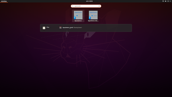
The installation scripts places two icons to the Desktop: vnmrj and vnmrjAdmin. vnmrj can either be launched by double-clicking on the desktop icon or from the command line:
1vnmrjIt is convenient to add Open VnmrJ to the quicklaunch menu. This can be done by by searching for “openvnmr” and then dragging the program icon to the quicklaunch bar.
OVJ-B12 is now installed and ready for its first experiment.
1.2.2 - Setting Up the Hardware
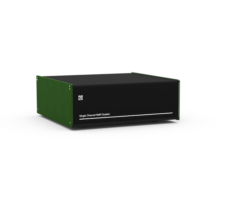
System Description
Front Panel Connectors
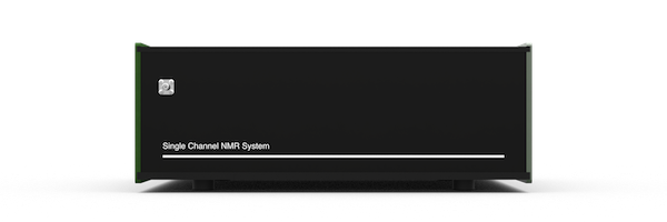
Bridge12 SCN Front Panel Connectors
The NMR probe is connected to the Bridge12 SCN using the SMA connector located on the front panel of the system.
Back Panel Connectors
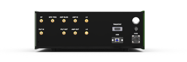
Bridge12 SCN Back Panel Connectors
Most connections for the Bridge12 SCN are located on the back panel.
| Connector Label | Style | Description |
|---|---|---|
| USB | USB-B | USB connection to spectrometer computer |
| PWR | Circular | System power connection. The input voltage for the system is 24 VDC, 1.25 A. To power the system, please use the power (desktop) adapter that was delivered with the system. |
| FILT IN FILT OUT |
SMA(f) | Receiver input filter (bandpass). The bandpass filter is used to reduce the noise in the system. By default the Bridge12 SCN comes with a bandpass filter for 1H NMR spectroscopy. If you like to operate the system at a different Larmor frequency the filter has to be replaced with a bandpass filter for the desired frequency. Additional filters can be found on the MiniCircuits webpage. |
| λ/4 | SMA(f) | Connection for the λ/4 cable. The Bridge12 SCN uses a passive Transmit/Receive (T/R) switch to protect the receiver. For this an appropriate λ/4 needs to be conneted to the two connectors. By default the system comes with a λ/4 cable for 1H NMR spectroscopy. If you wish to study other nuclei you need to replace the 1H with a cable with a different length. Instructions to make your own cable can be found on the webpage for the OpenTRSwitch or contact Bridge12 at support@bridge12.com. |
| AMP IN | SMA(f) | External amplifier input. |
| AMP OUT | SMA(f) | External amplifier output. |
| AMP BLNK | SMA(f) | Blanking gate for external amplifier. The blanking gate is active low. If you have questions about how to connect an external amplifier please contact Bridge12 at support@bridge12.com |
| MPS TRIG | SMA(f) | Trigger pulse for the Bridge12 MPS to modulate the output power. The trigger is active high. |
| SP | SMA(f) | Not used. |
| TRIG/STAT | D-Sub (f) | Auxiliary connector. Pinout: 1: 10 MHz reference for external use, 2, 3: Not connected, 4: Hardware trigger, 5: Hardware reset, 6, 7, 8, 9: GND |
Fuse
A fuse holder is located on the back panel of the SCN. If necessary, the user can replace the fuse. The dimensions are 5x20mm and the fuse should have a rating of 1.25A.
Placing the System
- Place the Bridge12 SCN close to the EPR spectrometer. It is recommended to keep the length of the cable connecting the probe to the system at a minimum length.
- The system should rest on a stable surface.
TRIG/STAT Channel Explanations
- 1 - 10 MHz Reference:
- The 10 MHz reference is the master oscillator output
- 4 - Hardware Trigger:
- When this is pulled to GND an acquisition resumes or starts
- 5 - Hardware Reset:
- When this is pulled to GND the pulse program is reset - as long as this is low no pulses are generated and sent out
- 6/7/8/9 - Ground
Connecting the System
Electrical Connections
To power the SCN connect the external power supply to the PWR connection. then connect the USB-C port to a PC. Connect the input of a bandpass filter corresponding to your NMR frequency to the ‘FILT OUT’ connector and the output of the bandpass filter to the ‘FILT IN’ connector. Connect a \(\lambda\)/4 filter (e.g. a cable with the correct length) for your NMR frequency to the \(\lambda\)/4 connectors.
Connecting the NMR Probe Circuit
Changing the RF Filters
Not sure if we need this right now.
1.2.2.1 - Connecting the NMR Probe
The connector to connect the NMR probe to the Bridge12 SCN spectrometer is located on the front panel. The input impedance is 50 Ω.
If your probe has a BNC connector please use a SMA-BNC Adpater and a BNC cable to connect the probe.
1.2.2.2 - Connecting an External Amplifier
The Bridge12 SCN has an internal RF power delivering up to 2 W output power. For many (low frequency) experiments this power is sufficient.
If the available power from the internal amplifier is not sufficient, an external high-power RF amplifier can be connected to the system.
To connect an external amplifier the input of the external device must be connected to the AMP OUT connection on the back panel of the SCN. The output of the external amplifier must be connected to the AMP IN connection located on the back panel.
To blank the external amplifier, connect the blanking gate to the AMP BLNK output of the SCN. The blanking gate is active low.
Specifying the Amplifier pre-Blanking Time rof1
To use an external amplifier with blanking, the amplifier needs to be unblanked before sending the RF pulse. Amplifiers typically require a short time unblank. This time can be specified using the OVJ parameter rof1. The value is typically given by the manufacturer in the data sheet of the amplifier.
The value can be set from the OVJ command line:
|
|
If the required value is larger than the default value, for rof1 can be changed using the setlimit command as shown below.
|
|
Enabling the External Amplifier and Setting the Drive Level
OVJ needs to be connected to use the external amplifier. This is done from the OVJ command line:
|
|
The B12SCNControl('state?) command can be used to query the state of the amplifier. If the system returns “extamp” the external amplifier is enabled.
|
|
The drive level (input power) of the external amplifier can be set using the OVJ command line by specifying the value stored by tpwrf.
|
|
To disable the internal amplifier from the OVJ command line enter this command:
|
|
If the command B12SCNControl('state?) returns “intamp”, the internal amplifier is used. The tpwrf value is automatically set to 100 (the maximum).
Warning
The drive level for the external amplifier is by default set to 3 dBm (2 mW - corresponding to tpwrf=3.25). This value can be changed using the tpwrf command from the OVJ command line. Please consult the data sheet of the external amplifier to find out the correct drive level for you amplifier model. The value in tpwrf is a linear scaling factor.
1.2.2.3 - External Trigger
The acquisition of an NMR spectrum by the Bridge12 SCN system can be triggered using an external trigger. The external trigger is connected to the TRIG/STAT connector located on the back panel. The pinout for the connector is given in the section describing the Back Panel Connectors.
The trigger is active low on the falling edge. This means, pulling pin 7 on the TRIG/STAT connector to GND will start the acquisition of an NMR spectrum. By default every acquisition needs to be triggered. If you require a different behavior (e.g. trigger 4 acquisitions to complete a phase cycle) the pulse program need to be changed accordingly. For further information please contact Bridge12 at support@bridge12.com.
The system also has a hardware reset, accessible through pin 9 on the TRIG/STAT back panel connector. When this pin is pulled to GND, the pulse program will reset. As long as the hardware reset of the SCN (pin 9) is pulled to GND no RF pulses are generated and send to the amplifier. Acquisition of an NMR spectrum is not possible.
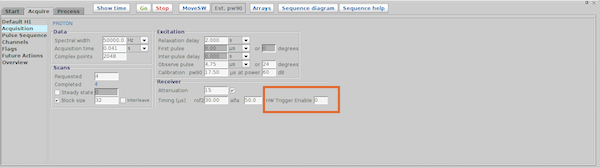
Enabling the External Trigger
The external trigger needs to be enabled in OVJ for the user to be used. This is done either:
-
from the OVJ command line:
1B12HWTriggerFlag=1 -
by setting the value in the Enable HW Trigger (in the Acquisition tab) to 1
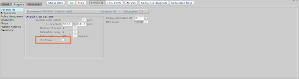
- or by activating the HW Trigger checkbox in the 1H tab
Disabling the External Trigger
To disable the external trigger use the command
|
|
or set the value in the Enable HW Trigger box to 0 (Acquisition tab) or disable the checkbox in the Default 1H tab.
1.3 - Getting Started
The following section gives an overview how to start OVJ, tune the probe to the correct frequency, and how to acquire a simple 1D 1H NMR spectrum.
1.3.1 - Launching OVJ
Launching OVJ
OVJ can be launched in two different ways: 1) by double-clicking the vnmrj icon on the desktop or, 2) by opening a terminal window and launching it from the command line by typing:
|
|
Setting the Spectrometer Frequency
If this is the first time you are using OVJ, the spectrometer frequency has to be set to the correct value.
Note
The first time you launch OVJ the spectrometer frequency has to be set. Once the spectrometer frequency has been set the value will be stored by OVJ and does not have to be entered every time the user starts OVJ.
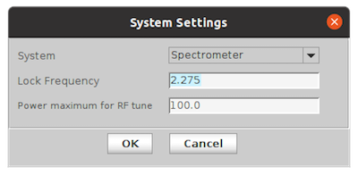
In OVJ, the spectrometer is historically set by setting the frequency of the deuterium (2H) lock frequency.
The ratio between the (1H) and (2H) frequency is approximately 6.51. For example, to set the spectrometer to a 1H frequency of 14.5 MHz the user has to set the spectrometer frequency to 14.5/6.51 = 2.227 MHz. To set the spectrometer frequency:
-
In OVJ go to Edit -> System Settings

-
In the window that appears enter the deuterium (2H) lock frequency in MHz.
Alternatively, the spectrometer frequency can be set from the OVJ command line using the lockfrequency parameter:
|
|
Next, you are ready to Tune the Probe.
1.3.2 - Tuning the Probe
Warning
The following section describes how to tune the NMR probe to the correct spectrometer frequency. This requires disconnecting the NMR probe from the spectrometer.
Make sure all experiments have been finished and no pulses are transmitted anymore before disconnecting the NMR probe from the spectrometer.
Tuning the NMR Probe
To tune the NMR probe to the spectrometer frequency follow these steps:
- Note down the spectrometer frequency. This does not have to be an exact value, but should be close (within 0.1 MHz of the operating frequency).
- Switch on the nanoVNA and set the center frequency to the spectrometer frequency (set it to the frequency of the nucleus you want to observe, not the 2H lock frequency). Set the span to a value of 1-2 MHz.
Note
See the page Setting up the Display to configure the nanoVNA for S11 measurements.
For instructions on how to setup the center frequency, span, marker position, etc. see the page with the setup instructions for the nanoVNA.
If this is the first time using the nanoVNA you should calibrate the device. This calibration needs to be repeated every time you change the center frequency or span.
- Disconnect the NMR probe from the Bridge12 SCN spectrometer and connect it to channel 0 (CH0) of the nanoVNA.
- You should see a ‘Tuning Dip’ on the nanoVNA. If you do not see a tuning dip try one of the following things:
- Increase the span of the VNA to scan a broader frequency range
- Change the matching on your probe
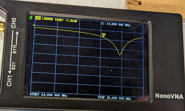
- Use the slider at the top of the nanoVNA to move the marker to the spectrometer frequency (within +/- 0.1MHz). The marker will tell you the absolute value of the S11 parameter at the spectrometer frequency (see image below, S11 = -7.8 dB).
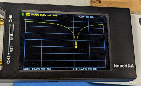
- Turn the tune and match capacitor of your probe to achieve a minimum reflection. In general, the tune capacitor will shift the dip up in down with frequency, while changing the match capacitor value will increase the depth of the dip. Optimize both capacitor values for a minimum in reflected power. The probe is tuned once you achieve the lowest value for S11 (see image below, S11 = -40.9 dB)
Next, you are ready to Acquire an NMR Spectrum.
1.3.2.1 - Using the nanoVNA
The Bridge12 SCN is delivered with the nanoVNA, a pocket-size vector network analyzer (VNA) to tune the probe to the transmitter frequency of the spectrometer.
The nanoVNA has two channel and has many different ways to display the (complex) S parameters. However, in the following we provide a brief set of instructions to setup the nanoVNA display to:
- Only show the reflected power from the probe (S11)
- How to calibrate the nanoVNA.
The nanoVNA will store these settings, so you only have to go once through these instructions.
For a complete reference please visit the nanoVNA Webpage.
Note
To navigate through the different menus of the nanoVNA you can either use the wheel located at the top of the device or using the touch screen. The touch screen is best used with a stylus pen.
Setting up the Display
To setup the display:
- Tap the touchscreen to show the menu
- Tap the Display button (top right corner)
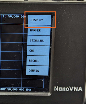
- Tap the Trace button on the display
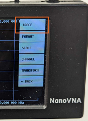
- For convenience, select only Trace 0 by tapping on it. The selected trace is highlighted with a colored background (yellow for Trace 0). Unselect any other traces by tapping on the button.
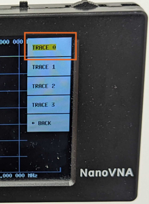
- To leave the menu tap somewhere on the touchscreen.
Setting the Frequency Range
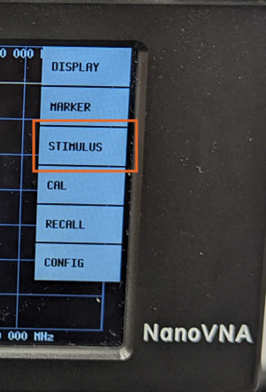
- Tap on the touchscreen to show the menu
- Tap on the Stimulus button
- Next, tap the Center button
- On the next screen, enter the spectrometer frequency using the number pad and press the M button to indicate that the entered frequency is given in MHz.
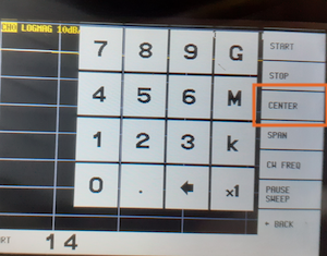
- Next, tap the Span button and enter the frequency range to observe the resonator tuning dip. Typically 1-2 MHz is a good range to start with.
Calibrating the nanoVNA
Important
The nanoVNA should be calibrated frequently. The calibration is only valid for a given set of parameters (e.g. span, center frequency, number of points ….). If one of these parameters is changed, the device needs to be recalibrated.
The device will still work even with a calibration that is “slightly off”. For example, the spectrometer frequency will not change drastically on a day to day basis and using the same configuration is ok. However, if you require accurate values for S11 we recommend calibrating the device before taking the measurement.
We recommend calibrating the device once and then not changing the measurement parameters. This should be good for a day-to-day operation.
The nanoVNA is calibrated using a basic OPEN-SHORT-LOAD protocol. Three SMA connectors are included with the nanoVNA, used for calibrating the device (see image below).
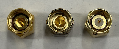
- SHORT - Left, used to shorten the input of the VNA. This connector is all metal on the inside.
- OPEN - Middle, used to create an open port. This connector does not have a middle pin.
- LOAD - Right, used to simulate a 50 Ω load. This connector has a middle pin and a white teflon ring around it.
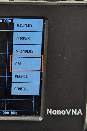
To calibrate the nanoVNA:
- Set the center frequency and span to the desired range by following the instructions above.
- Tab the Cal button on the display
- Connect the OPEN standard to the CH0 port and press ‘Open’
- The open entry is now black underlined
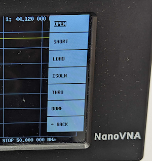
- Connect the SHORT standard to the CH0 port and press ‘Short’
- Connect the LOAD standard to the CH0 port and press ‘Load’
- Press ‘Done’
The nanoVNA is now calibrated.
Charging the Battery of the nanoVNA
From time to time the nanoVNA battery needs to be recharged.
To recharge the battery connect an USB-C cable to the nanoVNA and plug the cable either into a USB charger or a computer.
1.3.3 - Acquiring a Proton Spectrum
This section provides a brief overview how to acquire a 1D
- OVJ-B12 is installed on the computer
- The hardware is set up properly
- A sample is inserted into the probe
- The NMR probe is tuned to the spectrometer frequency.
Acquiring a 1H NMR
-
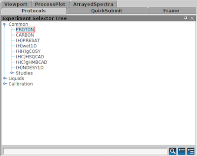
From the protocols tab drag the PROTON experiment into the plotting window, or double click on the PROTON protocol.
Alternatively, the pulse sequence can be set using the OVJ command line:
1seqfil='s2pul'The PROTON sequence calls a pulse program s2pul. This is a general, two-pulse sequence used to run variety of different experiments such as a single pulse NMR experiment or an inversion-recover sequence.
-
Next, the user has to set the length and power of the RF pulse to properly acquire a 1D 1H spectrum. In OVJ the pulse parameters can be changed from the OVJ command line or from the acquisition panel.
Note
Make sure that the spectrometer frequency is set correctly. The spectrometer frequency is set by adjusting the lockfreq. For experiments at 14.79 MHz, this parameter has a value 2.271 MHz (2H frequency corresponding to a 1H frequency of 14.78 MHz). This value should be ideally set to a precision of three to four significant digits.
See the Launching OVJ section in the Getting Started section for more details.
The length of the observe pulse is given by the parameter pw. From the OVJ command line set the pulse length:
|
|
corresponding to a pulse length of 3 µs.
Note
If the pulse length corresponding to a 90 degree pulse is unknown, it can be determined by performing a nutation experiment to calibrate the correct pulse length. Typically, the probehead manufacturer will provide the length and power level for the 90 degree pulse.
-
Next some of the acquisition parameters need to be set. Go to the Acquire tab and click on Acquisition. Here, basic acquisition parameters can be adjusted. Alternatively, the values can be entered in the OVJ command line.
- Spectral Width: Parameter sw
- Acquisition Time: Parameter at
- Complex Points: Parameter np
For example
1 2sw=50000 np=4096will set the spectral width to 50000 Hz (50 kHz) and the number of points acquired in the time domain to 4096.
Note
In OVJ the number of points corresponds to the total number of real and imaginary points. To acquire a total of 2048 (complex) points, np has to be set to 4096 (twice the number of complex points).
-
Set the number of transients (
nt) to 4. In general, OVJ will add a CYCLOPS phase cycle to each sequence automatically to remove DC offsets and correct for phase imbalances. Therefore, the parameterntshould always be set as a multiple of 4.1nt=4 -
On the Acquire tab click Channels to set the transmitter offset
tofparameter. To get started, set this value to 01tof=0With the transmitter offset set to 0, the spectrum, if excited on resonance, appears in the center of the window. To center the spectrum adjust the
tofvalue. Alternatively, you can click with the mouse on the peak (single red line cursor) and enter the commandmovetofin the OVJ command line. OVJ will automatically adjusttofso that the NMR spectrum in the next acquisition is at the center of the window. -
Start the acquisition by either pressing the GO button or by typing
1goin the OVJ command line. The acquisition will start and the data is displayed and processed on the screen.
Note
In OVJ the acquisition of the NMR spectrum can be started using the go or ga command. In this version of OVJ the two commands are identical. This may be different on other (older) NMR spectrometers running vnmrj.
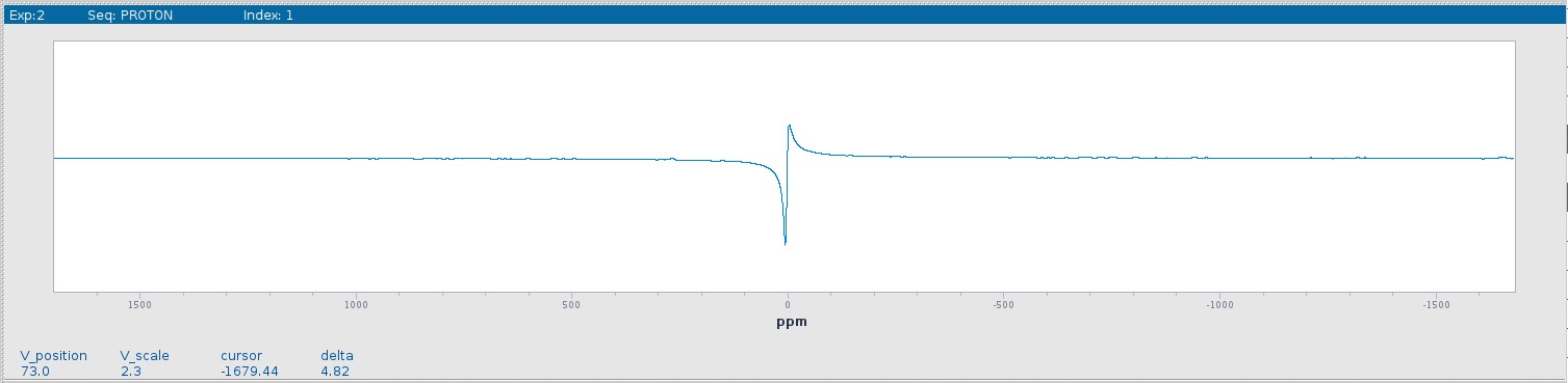
Phasing a spectrum
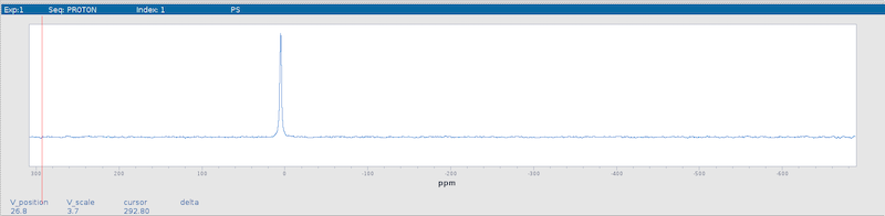
Once the acquisition is finished, the spectrum most likely needs to be phased to show just the real part of the complex spectrum (see figure below). This can be done automatically using the autophase command aph or manually.
Using the Autophase Routine
To autophase the spectrum type the following command in the OVJ command line and press enter:
|
|
to autophase the spectrum.
Manually Phasing the Spectrum
Sometimes, the autophase routine fails and the spectrum needs to be phased manually. To manually phase an NMR spectrum:
-
Click the Phase button in the toolbar to the left

-
Click the spectrum with the left mouse button and keep the button pressed. Two red cursors appear to the left and right of the peak. Phase the peak by moving the mouse up and down. This will adjust the 0th order phase correction (frequency-independent phase correction). Alternatively, the phase can be adjusted from the OVJ command line by typing:
1rp=11.5 -
To adjust the 1st order phase correction (frequency-dependent phase correction) click the Phase button in the toolbar to the left. Next, select the peak by moving the mouse cursor to the NMR peak and click the right mouse button. The point selected is the pivot point used to adjust the 1st order phase correction. By moving the mouse up and down the phase of the rest of the spectrum can be adjusted. To adjust the 1st order phase correction
lpfrom the OVJ command line type:1lp=157
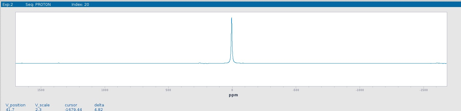
The proper phased spectrum is shown below.
Note
Start phasing the spectrum with rp and lp set to 0. First, adjust the 0th order phase and then the 1st order phase correction. Note that rp=360 is equivalent to rp=0. This is also true for lp.
Next, proceed to the next section to Save the NMR Spectrum.
1.3.3.1 - Processing 1D Spectra in DNPLab
DNPLab is a Python package to process NMR data. The software was developed by Bridge12 and is open-source, free to use. DNPLab can be used for offline processing of OVJ data.
Below, a brief example is shown how to load and process a 1D NMR spectrum. For a complete reference and many more processing examples visit the DNPLab Online Documentation.
Installling DNPLab
DNPLab requires a working Python installation and can be simply installed using pip:
|
|
All requirements are automatically installed.
Processing 1D Spectra
A typical processing and plotting script is shown below:
|
|
The general structure of the script is:
- Line 1: Import the DNPLab package.
- Line 3: Load the NMR spectrum. DNPLab can import many different spectrometer formats. The format is automatically detected and a dnpdata object is created.
- Line 4: The attribute of the spectrum needs to be changed to nmr_spectrum to ensure that the plot function
fancy_plotworks properly (this line will not be required in the future). - Line 6-7: Fourier transform the spectrum and apply an autophase routine.
- Line 8: Remove DC offset from spectrum.
- Line 10-11: Plot the NMR spectrum
The result is shown below.
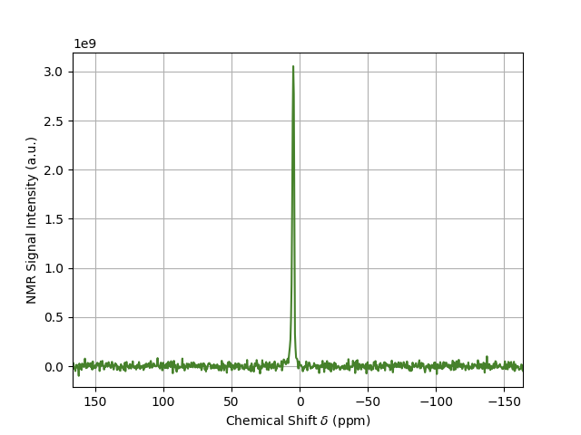
DNPLab has many more features for processing and analyzing NMR data. It can also be used to process EPR data. For more information check out the Online Documentation.
1.3.4 - Saving the NMR Spectrum
OVJ provides two different options to save the NMR data:
- by using the OVJ GUI
- by using the OVJ command line.
Saving Data using the OVJ GUI
To save the NMR experiment using the GUI:
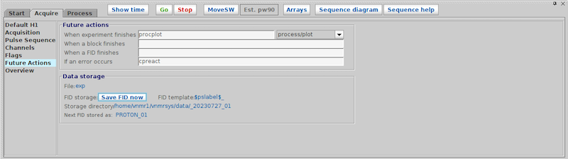
- Go to the Acquire Tab and select Future Actions
- Click on save FID (see image below)
Saving Data from the OVJ Command Line
To save the NMR experiment from the OVJ command line:
- Type the command
save - Enter a name (e.g. mydata). Do not add an extension to the file name
- Press return
The data will be saved and a study is created automatically.
Location of Saved Data
Assuming a default installation of OVJ, the data can be found in the ‘mydata’ subfolder in the vnmrsys/data folder:
|
|
1.4 - Advanced Experiments
This section provides some examples of advanced experiments and data acquisition schemes.
1.4.1 - Arraying Parameters
For many experiments a parameter needs to be varied (e.g. the delay (recovery) time in an inversion-recovery experiment to measure the 1H longitudinal relaxation time T1.
In OVJ, this can be done specifying an array of parameters. An array can be either specified through an OVJ GUI or the command line.
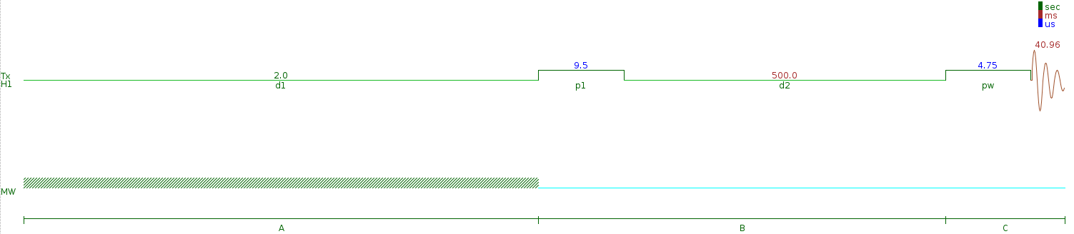
It is helpful to first take a look at the pulse sequence to decide, which parameter needs to be arrayed. Either click the ‘Sequence diagram’ button in OVJ or type dps in the OVJ command line. A typical, two pulse experiment is shown in the figure below.
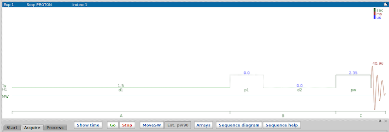
- d1: Repetition time.
- p1: Pulse length of the first pulse. For an inversion recovery experiment, this is the pulse length of the first 180 degree pulse.
- d2: Recovery delay.
- pw: Pulse length of the detection pulse.
Arraying Parameters using the GUI
To use the GUI to define an array of parameters to vary follow these steps:
-
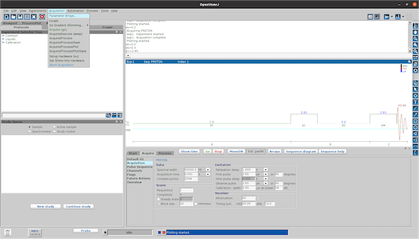
In the Acquire Tab click the array button or select Parameter Arrays from the Acquisition menu
-
In the window, enter the parameter name to array in the field Param Name. In this example we will vary the parameter
d2. The description will be automatically filled in.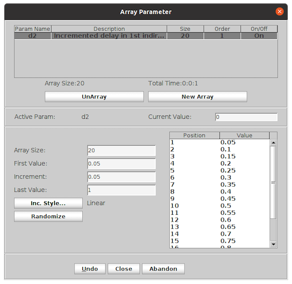
-
Enter three of the four parameters (Array Size, First Value, Increment, Last Value). The fourth parameter will be calculated once three values are entered.
The values of the array is shown in the box to the right. Use the scroll bar see all values of the array.
-
Click the Close button.
The window will close. The value of the parameter (here
d2) will now be displayed as “Array” to indicate an array of values instead of a single value.
Arraying Parameter using the OVJ Command Line
From the OVJ command line, an array can be defined using the array command.
|
|
For example, to array the parameter d2, starting at 0.05 s, with steps of 0.05 s for a total of 30 points enter the following command:
|
|
another possibility to create arrays with arbitrary values is using the syntax $value=val1,val2,…
|
|
1.4.2 - Calibrating the 90º Pulse Length
Calibrating the 90º pulse length is a good example for arraying parameters in OVJ. If you haven’t read the section about how to array parameters in OVJ, we would suggest doing this first before you start to follow this example.
To calibrate the 90 degree pulse length follow these steps:
- Insert a water sample into the probe.
- Select the PROTON sequence in OVJ.
- Set the following parameters in OVJ.
- Set the sweep width (
sw) to a value that the NMR signal (here a single peak from the water sample) is fully within the sweep width of the experiment and some noise is shown left and right to the peak. - Set the number of scans (
nt) to a value to obtain a clear signal (not too noisy). - Set the number of acquired points
npto 4096, to acquire 2048 complex points.
- Set the sweep width (
- Array the parameter
pwfrom 0 to about three times the expected pulse length for the 90 degree pulse. In this example we set the array the parameter from 0 to 15 µs with a step size of 0.25 µs. - Start the acquisition of the experiment and save the data once the experiment has finished.
The obtained data can be either analyzed in OVJ or dnplab to determine the length of the 90 degree pulse.
Determining the 90 Degree Pulse Length in OVJ
To process the nutation experiment in OVJ follow these steps:
-
After the acquisition select the ‘Process’ tab
- Select Display and set the display mode for the spectrum to ‘Phased’
- Select a spectrum that with sufficient signal-to-noise and phase the spectrum. Use a spectrum with a shorter pulse length, don’t use the last spectrum of the nutation experiment. The same phase correction is applied to all spectra in the array.
-
If the sweep width of the spectrum is large, zoom into the region with the peak.
- Move the mouse cursor to the left of the peak and press the left mouse button. Next, move the mouse cursor to the right of the peak and click the right mouse button. The selected region is shown between the two red lines.
- Click on the zoom button in the toolbar to the left to zoom into the region defined by the two red lines.

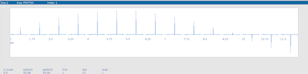
-
To show all spectra horizontally aligned, together with their respective pulse length
- Press the |||| button to show all spectra next to each other

- Next, click # to cycle through the acquisition number or the array parameter

-
To show all spectra of the array press the # button in the toolbar
-
The spectrum with the largest peak corresponds to the 90 degree pulse width. In this example the optimum pulse length is 4.75 µs.
Determining the 90 Degree Pulse Length in DNPlab
The nutation experiment can also be analyzed in DNPLab. If you haven’t installed DNPLab, this can be easily done using pip:
|
|
A typical DNPLab script to determine the 90 degree pulse length is given below:
|
|
This processing script first will load the data and does a Fourier transformation of the FID. Next, a DC offset will be removed using the remove_background function. Next, the NMR peak intensity is integrated using the integrate function and the data is plotted using the fancy_plot function.
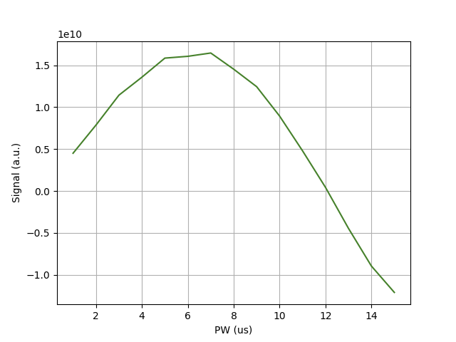
In the example the 90 degree pulse length is about 2.35 µs, and the 180 degree pulse length is about 4.7 µs.
Note
Different probes will have different pulse lengths for the 90 degree pulse. The pulse length also depends on the RF power. Higher RF power will result in a short pulse length. However, you should not exceed the maximum pulse power specified by the manufacturer to avoid damaging the probe.
1.4.3 - Inversion Recovery Experiments in OVJ
The longitudinal relaxation time T1 can be determined from an inversion-recovery experiment. This is another good example to demonstrate the arrying capabilities in OVJ. If you haven’t read the section about how to array parameters in OVJ, we would suggest doing this first before you start to follow this example.
The following pre-requisites are assumed:
- A sample is inserted in the probe.
- The 90 degree pulse length is know. To determine the correct pulse length please follow the steps outlined in the section Calibrating a 90º Pulse.
Acquire the Inversion Recovery Data
To perform the inversion-recovery experiment follow these steps:
-
Select the PROTON experiment (
seqfile='s2pul'). -
Enter the pulse for the 90 degree pulse (pw) and the 180 degree inversion pulse (d1).
-
Enter a value for d1. This is the repetition time of the experiment and it should typically be set to a value of 5 times the T1 relaxation time of the nucleus. For example, if the relaxation time of the water protons is about 1 s, the value for d1 should be set to 5 s. This ratio can be reduced to speed up the experiment, however, if the repetition time is too short, the measured value for T1 will be incorrect.
-
For the inversion-recovery experiment we will array the d2 parameter
1array('d2',30,0.05,0.05) -
Press ‘Go’ to start the acquisition or type
goand press enter in the OVJ command line. -
Once the aquisition is finished save the data.
Determining T1 in OVJ
To determine T1 in OVJ follow these steps:
-
Select the last spectrum of the array using the
dscommand. Here, we use spectrum number 15. Alternatively, you can select any spectrum with sufficient signal-to-noise.1ds(15) -
Phase the spectrum using the autophase function
aph:1aphOnce all spectra are phased, you can display all spectra horizontally using the
dsshcommand:1dsshThe result should like like the example below
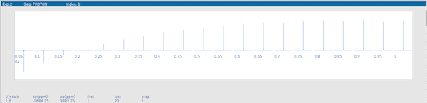
If the spectra look like the data shown in the image proceed to the next step.
-
Select the last spectrum using the
ds(15)command. -
Next, we need to set a threshold for the peak picking algorithm. The threshold is set using the
thparameter. In this example, we will set a threshold of 10.1th=10You can also use the horizontal line marker to adjust a threshold. Set the threshold to a value that only one peak is above the threshold.
-
In the next step the peak amplitudes for each spectrum are determined using the
dllandfp(find peak) command. Only peaks are considered that are above the threshold value.1 2dll fp -
To get the T1 relaxation time, the t1 OVJ macro can be used. To run the macro, enter t1 in the OVJ command line and press enter.
1t1 -
Display the fitting results using these OVJ command line commands:
1 2center explYou should see a result similar to the one shown below.

The fit values returned by the t1 macro can be seen in the Process tab under Text output.

The t1 macro will create an output file located in the current experiment folder. The path the folder is (N corresponds to the experiment number). The number of the current experiment can be seen in the top left part of the display tab or using the curexp? command in the OVJ command line.
|
|
Evaluation with dnplab
The inversion-recovery experiment can also be analyzed using DNPLab. First, make sure DNPLab is installed:
|
|
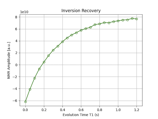
A typical processing script is given below:
|
|
The first subfigure can be used to determine the noise and signal region. The second figure shows the T1 recovery curve. An example for the second figure is shown below.
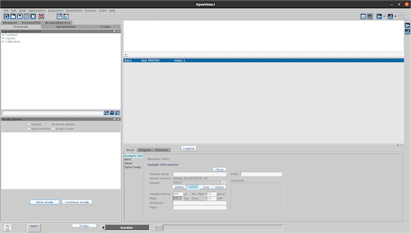
1.4.4 - Creating a Study in OVJ
If the user wants to run a series of experiments a Study should be created in OVJ by the user. The study can be started using the go command and each experiment is automatically saved.
To create a study in OVJ follow these steps:
-
Click ‘New study’ in the ‘Study Queue’ tab.
-
Enter a Sample name in the ‘Start’ tab.
-
Drag an experiment (e.g. PROTON) from the Experimentor Selector Tree into the Study Queue.
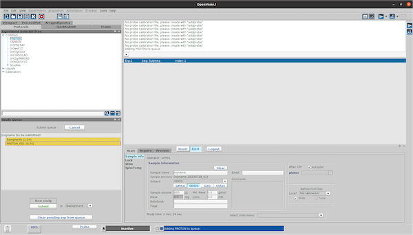
when the the PROTON_001 sequence is selected (double click) one can adjust all settings for the sequence (Array parameters, change MPS settings, etc..) and when pressing the save button the settings are saved.
These settings will be the default settings for all experiments in this study. To save the data automatically go to the ‘Acquire’ tab and select ‘Future Actions’.
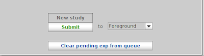
-
In the ‘When experiment finished’ line enter procsaveplot (select process/plot/save from the dropdown menu) or save to save the data after each ‘go’. Alternatively this can be set with the commandline
1wexp='procsaveplot' -
To start the acquisition of experiments in the study, press the Submit button to start the acquisition.
1.5 - DNP Experiments using OVJ
(Overhauser) DNP-enhanced NMR experiments can be conveniently performed in OVJ. Here, OVJ not only controls the NMR hardware, but also the Brigde12 Microwave Power Source (MPS). From OVJ it is possible to:
- Control the power and frequency of the MPS
- Record the tuning dip of the microwave cavity
- Vary acquisition parameters (e.g. microwave power) automatically
In this section we demonstrate a couple of simple DNP experiments and how to incorporate automating the MPS control into OVJ pulse programs.
1.5.1 - Controlling the MPS from OVJ
The Brigde12 MPS can be completely remote controlled from within OVJ. Make sure, the MPS is connected to the computer running OVJ using a USB cable.
The Bridge12 MPS is controlled from a dedicated panel within OVJ. To access the panel:
- Select the tab label Start from the panel
- Click on MPS to access the panel
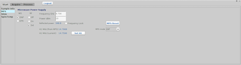
Most controls in this panel are labeled identically to the front panel labels of the MPS.
- WG: This check box controls the waveguide status. OVJ will allow the use to only check one box at a time. For example, if the DNP box is checked, the EPR box will be unchecked and vice versa.
- RF: This check box controls the microwave power output status:
- Off: The microwave power is disabled
- On: The microwave power is enabled
- Ext: The MPS is waiting for an external trigger signal to enable the microwave power
- Frequency (GHz): Microwave frequency in GHz
- Power (dBm): Microwave power in dBm. If your are not familiar with the dBm scale, a conversion table is available in the MPS documentation
- Reflected power: The value printed here indicates the amount of reflected power from the cavity.
- Frequency lock: This check box enables the software-AFC feature of the MPS.
- MPS Reset: This will trigger the MPS to reboot.
OVJ calculates the 1H frequency from the microwave frequency that the MPS is set to. It is displayed as H1 MHz (from MPS). The frequency is given in MHz. Under it, the current OVJ 1H frequency is given. In most cases, these two values should be close. To set the spectrometer frequency to the calculated 1H frequency from the MPS, hit the button labeled Set H1.
1.5.2 - 1H ODNP Spectroscopy
In this first example we demonstrate how to record an NMR spectrum with and without microwave power. Here, it is assumed that the microwave resonator is properly connected to the MPS, and that the resonator is properly tuned and matched.
Warning
Before enabling the microwave power on the MPS, make sure the microwave resonator is properly coupled to the MPS. While the MPS has a safety feature to disable the microwave power if the reflected power exceeds a safe value, exceeding this value can cause permanent damage to the MPS.
The NMR signal recorded without microwave power is often referred to as the Off Signal, or the thermal equilibrium (TE) signal, while the signal recorded with microwave power is often referred to as the On Signal. In most cases, optimizing the spectral parameters using the On Signal is simpler due to the increased signal-to-noise of the spectrum.
Sample: For this example we use a sample of 10 mM TEMPO dissolved in water. The sample is loaded in the appropriate sample tube and inserted into the resonator.
Prior to recording a DNP spectrum the user has to:
- Adjust the microwave coupling to minimize the reflected microwave power.
- If necessary, record an EPR spectrum of the sample
- Adjust the magnetic field strength so the microwave radiation is on-resonance with an EPR transition
Recording the On Signal
To record the On Signal:
- Select the PROTON experiment (seqfile=‘s2pul’) and set the NMR acquisition parameters ((nt, sw, tof, np, d1, pw, etc.) to some common values.
- Go to the Start tab and select the MPS panel.
- Select the DNP checkmark (under WG) in the MPS tab. This will set the waveguide switch to select the microwave path for DNP. A waveguide switch is commonly installed in systems that are based on an EPR spectrometer. Your system configuration may differ.
- In the MPS panel, enter the microwave frequency. This is the same frequency that the EPR resonator is tuned to.
- Enter the microwave power (see this table for conversion of mW to dBm). The power requirement for a DNP experiment strongly depends on the nature of the sample. A good starting value is 23 dBm (200 mW).
- Make sure the MPS mode is set to Manual.
- To enable the microwave power, click on the On check box under RF.
- Acquire an NMR spectrum by clicking the go button or by typing the
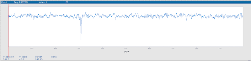
gocommand in the OVJ terminal. - Phase the spectrum. Note: Typically, the off-signal is phased so the NMR signal has a positive amplitude. In an ODNP experiment, the enhanced peak will be inverted.
The ODNP-enhanced spectrum is shown in the figure below.
Next, optimize the acquisition parameters of the NMR experiment.
Recording the Off Signal
Once the acquisition parameters are optimized you can record the off-signal, the NMR signal without microwave power. Typically, the signal-to-noise ratio will be much lower and often more averaging is required. To record the off-signal:
- Turn off the microwave power by clicking the Off check box under RF.
- Acquire an NMR spectrum by clicking the go button or by typing the
gocommand in the OVJ terminal.
If the signal-to-noise ratio is not sufficient, increase the number of acquisitions (OVJ parameter nt).
Keep in mind, to calculate the DNP enhancement, either both, the on and the off spectrum have to be recorded with the same number of transients, or the signals have to be properly normalized.
1.5.3 - DNP Power Build-UP (Saturation) Cruve
A commonly performed DNP experiment is to record the NMR signal intensity with respect to the microwave power. The result is the DNP power saturation behavior.
In this example we will automatically record the DNP saturation curve for a sample of 10 mM TEMPO in water.
To record the DNP saturation experiment:
-
Select the PROTON experiment (seqfile=‘s2pul’) and set the NMR acquisition parameters ((nt, sw, tof, np, d1, pw, etc.) to some common values.
-
Connect the MPS TRIG output to the MPS Ext. Trig input using a BNC cable.
-
Go to the Start tab and select the MPS panel.
-
Select the DNP checkmark (under WG) in the MPS tab. This will set the waveguide switch to select the microwave path for DNP. A waveguide switch is commonly installed in systems that are based on an EPR spectrometer. Your system configuration may differ.
-
In the MPS panel, enter the microwave frequency. This is the same frequency that the EPR resonator is tuned to.
-
Select Ext. mode from the MPS mode dropdown menu.
-
We will use continuous microwave radiation during the experiment. To turn the microwave power on permanently during the experiment set the xm variable to the value ‘yyy’
1xm='yyy' -
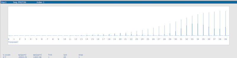
Next, we will create an array in OVJ with the microwave power values. For this the parameter mpspower needs to be arrayed. Create an array from 0 to 40 with a stepsize of 1, resulting in a total of 40 elements.
Note
Keep in mind a microwave power level of 0 dBm corresponds to 1 mW of microwave power, not 0 mW.
-
Start the experiment by clicking the go button or by typing the
gocommand in the OVJ terminal
Once the experiment is finished, the results can be conveniently displayed using the dssh command
1.5.4 - Using the External MPS Trigger
The Bridge12 MPS microwave source can be controlled by an external trigger to enable and disable the microwave power programmatically through the NMR pulse sequence.
To be able to use the external trigger, connect the MPS TRIG output from the SCN backpanel to the MPS Ext. Trig input of the MPS backpanel, using a BNC cable.
To enable the external trigger:
- Select a pulse sequence.
- In the MPS panel select the Ext mode from the dropdown menu.
- Select the checkmark Ext under RF
Now, the MPS is set to accept an external trigger signal. In this mode the RF output set by the status() command during the pulsesequence. In OVJ, every pulse sequence is divided into three different sections, labeled A, B, and C. This label is shown in the bottom row when displaying a pulse sequency in OVJ using the dsp command.
The microwave status (on or off) for these sections is controlled by the xm variable in the pulse program.
|
|
To enable the microwave power during Status(A) in the pulse program, but disable the power during Status(B), and Status(C) the xm variable has to be set to
|
|
When only a single character is given the status() is set for A,B,C to the same value.
When the xm variable is set, the status can be seen in the display of the pulsesequence by typing
|
|
An additional line labeled MW appears, indicating the status of the microwave output during each segment of the pulse sequency. In this example, the microwave power is enabled (ON) during Status(A) but disabled during Status(B), and Status(C).
Note that the position of the status() statement in the pulsesequence determines where a state starts and ends. As an example the following modified ‘s2pul’ includes p1 in status A and pw in status B
|
|
1.6 - Reference
1.6.1 - OVJ Commands
General Command Structure
- OVJ commands are entered at the command line. Some commands require arguments or parameters, which can enclosed in parentheses.
- To change a parameter value, the parameter is entered followed by an equal sign (=), followed by the value of the parameter (real, integer, or string).
- String values are always enclosed in parentheses and surrounded by single quotes.
- Multiple command and parameter settings can be entered consecutively, separated by spaces.
Command Examples:
|
|
Example of Setting a Parameter Value:
|
|
Commonly Used OVJ Parameters
The following sections provide a list of commonly OVJ commands and parameters. For a complete list of commands see the VnmrJ Command and Parameter Reference.
Commands
Spectrometer Control and Data Acquisition Parameters
| Command | Description/Example |
|---|---|
| aa | abort current running experiment immediately. Recommended to use in most occasions over sa except when some experiments are queued |
| cexp(n) | create new experiment from current one Example: cexp(2) copy current parameters and create experiment number 2 (#2 must not exist) |
| dg | display group of acquisition/processing parameters in Process→Text Output window |
| dps | display pulse sequence |
| ga | start experiment and autoprocess the data when data are available |
| go | start experiment using acquisition parameters |
| jexp(n) | join (or go to) specified experiment Example: jexp(2) join exp#2. exp#2 must exist |
| movesw | move new spectral window (sw) to the area enclosed by the two red cursors |
| movetof | move transmitter offset freqeuency (tof) to the cursor position |
| su | setup experiment. Force hardware to changes according to current parameter settings Example: load=‘MySpectrum’ su - change shims to current values in parameter file Example: tn=‘C13’ su - change direct detection to C13 |
| time | displays total experiment time with current parameters |
| time(hours,minutes) | displays number of scans (nt) required for a given time of experiment Example: time(1,10) - displays number of scans needed for a one hour 10 mins experiment |
| unlock(exp_number) | remove interactive lock and join an experiment. Useful to remove lockup of an experiment, sometimes due to user failure to exit vnmrJ before logging out Linux |
Data Processing and Display Commands
| Command | Description/Example |
|---|---|
| aph | automatic phasing of both zero (constant) and first-order (linear with frequency) terms |
| aph0 | automatic phasing with zero-order term only to achieve absorptive mode spectrum. Zero-order phase value (rp) is the same across the spectrum |
| array | Enter this command to set an arrayed experiment where a parameter is varied and an experiment is collected with each parameter. Enter parameter name, initial value, number of steps, and stepsize. All other parameters are kept constant |
| bc | 1D or 2D baseline correction with a spline or 2nd to 20th order polynomial function. Needs to define baseline regions (regions in between the integral areas covering peaks) |
| centersw | With full spectrum displayed and in single cursor mode, centers moves the cursor to the center (transmitter) of the spectrum |
| cz | clear integral reset points |
| da | display acquisition parameter array in Plot→Text Output window |
| dc | Apply a simple drift correction (with a straight line function) so that the spectrum baseline is close to zero. Level (lvl) and tilt (tlt) parameters are adjusted |
| df | display a single FID (default index is 1) Example: df displays the 1st FID or df(10) displays #10 FID in the array |
| dli | display list of integrals |
| dll | displays line frequency and intensities (peaks have to picked) |
| dpir | display integral values below spectrum |
| dpf | adjust threshold and display peaks so that a maximum 20 highest peaks are found and the minimum height cutoff is 5 times above noise level |
| dres | calculates peak resolution/linewidth |
| ds | display processed spectrum without preprocessing |
| dssa | display arrayed spectra in a stack plot Example: wft dssa |
| dssh | display arrayed spectra horizontally Example: wft dssh |
| dssl | Label displayed arrayed spectra with index number Example: wft dssh dssl |
| dsn | measure and display signal-to-noise ratio in region enclosed by two cursor lines |
| f | display the full spectrum |
| fbc | apply baseline correction for each spectrum in an spectrum array |
| full | display spectrum with full window size. The range of the spectrum is not changed Example: f full - display the full spectrum with full window size |
| fp | find peaks in arrayed dataset according to the refrence peaks found by dll |
| isadj | automatic adjustment of integral vertical display height to fit page |
| mf | move FID file from one experiment to another Example: mf(1,2) move fid from exp #1 to #2 |
| mp | Move all parameters from one experiment to another Example: mp(1,2) |
| nl | move cursor line to nearest peak/line position |
| th | set a threshold for peaks in dll command |
| thadj(maxpks,noise_mult) | Adjust the threshold th so that no more than maxpks number of peaks are found with a minimum of noise_mult factor above noise level. Example: thadj(20,5) |
| peak | Find tallest peak in current display region Example: peak - display tallest peak position and height in current displayed spectrum region Example: peak:$height,$freq - find tallest peak in current displayed region and save height and frequency in the variables $height and $freq. $heigt? or $freq? shows the values |
| vsadj | automatic vertical scale adjustment so that the highest peak fits the window height |
| setref | set reference ppm of any nucleus by the chemical shift of the deuterium signal from the solvent, according to IUPAC standard indirect referencing to TMS 1H signal |
| wft | Weighted Fourier transform (FT). Weighting is applying a window function to the profile of the FID to enhance resolution or signal-to-noise and to reduce truncation artifacts from finite data collection |
Plotting Commands
| Command | Description/Example |
|---|---|
| page | submit plot to printer and change plotter page. Usually last command in printing command chain |
| pap | plot “all” parameters in table format |
| pir | plot integrals below spectrum |
| pl | plot spectrum |
| pll | plot frequency line list in a table format |
| pltext | plot user comment/notes. Not necessary if ppa command is used |
| ppa | plot basic parameters in plain english format |
| pps | plot pulse sequence |
| ppf | plot peak frequencies over the spectrum |
Parameters
Acquisition parameters
| Parameter | Description/Example |
|---|---|
| at | acquisition time in seconds |
| bs | block size of data (number of transients) periodically read and stored on disk Example: bs=4 stores data every 4 scans |
| ct | current transient (or scan) number. ct is displayed at the bottom of vnmrJ screen during a running experiment. If the experiment is stopped before all transients are done, ct (stored in the parameter file procpar) is the number of scans completed |
| d1 | 1st delay period in pulse sequence. Typically this is the recycle time (in seconds) between scans |
| dn | 1st decoupler nucleus |
| gain | receiver gain. If gain=‘n’, auto-gain adjustment is set before data acquisition. Autogain cannot be used for arrayed experiment. Gain values go from 0 to 60. Too high a gain setting causes receiver overflow, leading to severe artifacts in the spectrum Example: gain=36 sets gain to 36 |
| nt | number of transients or scans |
| pad | preacquisition delay (in seconds). pad is the additional delay time set before the 1st recycle delay (d1) before the start of an experiment. If pad=60, the experiment will start after 60 secs |
| rattn | receiver attenuation, the attenuation can be set from 0 to 95, a too high value will attenuate all signals. A too small value will increase noise without increasing the signal strength. |
| ss | number of steady-state transients or dummy scans before start of experiment. It’s used to establish a steady-state for the spins before data collection |
| sw | spectral width of direct detection dimension, in Hz be default Example: sw=6000 or sw=15p to specify 15ppm width |
| sw1 | spectral width of 1st indirect detection dimension, in Hz be default |
| solvent | name of solvent Example: solvent=‘cdcl3’ or solvent=‘c6d6’ |
| tn | observe transmitter nucleus |
| tof | observe transmitter offset (center of spectrum) |
Processing and display parameters
| Parameter | Description/Example |
|---|---|
| axis | axis label in display and plots. Values include ‘h’ for Hz, ‘p’ for ppm Example: axis=‘p’ or axis=‘ppm’ set axis to ppm display |
| cr | cursor position in direct detected dimension Example: cr=8.0p set cursor position to 8ppm |
| date | date of experiment |
| delta | In two-cursor (box cursor) mode, delta stores the width in Hz between the two cursors Example: delta=1000 sets the separation between two cursors to 1000 Hz, or delta? to see the cursor separation value |
| ho | horizontal offset (in mm) between a set of spectra in stacked display mode for arrayed spectra |
| intmod | integral display mode. Value is ‘off’, ‘full’, or ‘partial’ Example: intmod=‘off’ |
| lb | line broadening amount for exponential weighting function (Hz) Example: lb=0.2 |
| lp | 1st order (or linear) phase in directly detected dimension, adjusted during phasing process Example: lp=0 sets linear phase correction to zero, useful to reset linear phase to zero to correct accidental introduction of large lp value during manual phasing |
| rp | zero order phase correction in degree, adjusted during phasing process Examples: rp=45 set zero-order phase to 45 degree or rp=rp+45 to change phase by 45 degree |
| vo | vertical offset (in mm) between a set of spectra in stacked display mode for arrayed spectra |
| vp | vertical position of spectrum, in mm Example: vp=60 sets spectrum baseline roughly in the middle of the display along Y-axis Example: vp=vp+20 moves the spectrum up by 20 mm |
| vs | vertical scale of spectrum Example: vs=vs*2 - set vertical scale to double peak height Example: vs=vs*0.5 - set vertical scale to halve peak height |
1.6.2 - Pulse Programming
General Concept
Pulse sequences are written in C, a high-level programming language that allows considerable sophistication in the way pulse sequences are created and executed.
A new pulse sequence is written as a C function called pulsesequence. The file containing this function is compiled and linked with an object library that contains the definitions for all pulse-sequence statements, the PSG. A compiled C sequence is executed on the Linux workstation at the start of acquisition, so-called run-time. At run-time, the sequence reads values from a parameter table and constructs a second real-time program of acodes, whose purpose will be to run the SpinCore controller board.
The PSG library contains C code to run the pulsesequence function and to run spectra corresponding to arrays of parameter values. The user need not program these loops explicitly. At the start of the acquisition, all of the variables and statements of the compiled C program, including the C loops and conditionals, are resolved and fixed into acodes, without the possibility of further input or calculation. A complex program with many choices, using the C if-else-endifstatement, may resolve into a very few acodes, because the acodes in the non-selected branches are never created. A pulse program with multidimensional looping and/or parameter arrays will produce a separate set of acodes for every increment.
The real-time acode program is automatically looped over the number of scans for each multidimensional increment or array element. Special real-time integer tables, t1 to t10, are used to increment phases and other values that might change scan-to-scan. These tables and variables are initialized and manipulated by special pulse-sequence statements, the real-time math statements.
Writing pulse sequences
Pulse sequence text files are stored in a directory named psglib in either the system directory (/vnmr/psglib) or in a user directory (/home/vnmr1/vnmrsys/psglib for the user vnmr1). A pulse sequence file has the extension .c to indicate that it contains C language source code. Pulse sequences may also be saved in the psglib directory of an applications directory, which may have any name and path. An applications directory is made accessible through the Edit Applications tool of the Files pull down menu. A pulse sequence text file can be modified using the Linux tool vi, the standard Linux editor gedit, or by an available text editor or development package.
The template for all pulse sequences is:
|
|
Since it is a C function, any C construction may be used. The available pulse elements are described below. For examples, see the pulse sequences in /vnmr/psglib
Compiling pulse sequences
After writing a pulse sequence, the source code is compiled by one of the following methods:
- By entering
seqgen(filename<.c>)on the OpenVnmrJ command line. - By entering
seqgenon the OpenVnmrJ command line, with seqfil=‘filename’ - By entering
seqgen filename<.c>from a Linux shell
For example, enter seqgen('s2pul') to compile the s2pul.c sequence in OpenVnmrJ. A full path is not necessary from the command line. Alternatively, you can enter
|
|
in a Linux shell. The seqgen command will first search the user, then the available applications directories, and then the system for a file with a .c extension.
During compilation, the system performs the following steps:
- Extensions are added to the pulse sequence to allow a graphical display of the sequence, using the dps command.
- The source code is checked for syntax, variable consistency, and the correct usage of functions.
- The source code is converted into compiled object code.
- If the conversion is successful, the object code is combined with the necessary system PSG object libraries (libparam.so and libpsglib.so), to be linked at run-time. If the compilation of the pulse sequence with the dps extensions fails, the pulse sequence is recompiled without the dps extensions.
The executable code is stored in the user seqlib directory (e.g. /home/vnmr1/vnmrsys/seqlib). If the user does not have a seqlib directory, it is automatically created. A copy of the source code is also saved in vnmrsys/seqlib of the user directory. If desired, you can copy the compiled sequence to /vnmr/seqlib or to the seqlib directory in an applications directory.
Standard compiled sequences are supplied in /vnmr/seqlib and the source code for each of these sequences is found in /vnmr/psglib. To recompile one of these sequences or to modify it, first copy the sequence into the user psglib, make the required modifications, and then recompile the sequence using seqgen. Sequences can only be compiled from a user directory. If you attempt to compile a system sequence, a local copy will be created. The seqgenupdate command performs a seqgen as the first step, and will then attempt to move the resulting seqlib entries back to the application directory from which they were taken.
The source files that are used to create the PSG object library are contained in the system directory /vnmr/psg. In principle, a user can customize and recompile the PSG source files, but most users do not do so. It is easier to add the user source code in a separate file using the standard C #include statement. User #include files should be stored in the ~/vnmrsys/psg directory of a user or an applications directory.
1.6.2.1 - Pulse Elements
Pulse sequences are constructed from pulse elements, which specify controls for the NMR hardware. The “C-style” signature for these elements is defined below.
Delay
|
|
Examples:
|
|
Pulse
|
|
|
|
Rgpulse
|
|
|
|
Offset
|
|
Acquire
|
|
|
|
Power
|
|
Settable
|
|
Status
|
|
|
|
Getstr
|
|
|
|
Getval
|
|
|
|
1.6.2.2 - Phase Cycling
There are several phase variables that control the phase of RF pulses and the phase of the receiver. These are:
- zero, one, two, three
- t1, t2, t3, t4, t5, t6, t7, t8, t9, and t10
- oph
The constants PH0, PH90, PH160, PH270 are used to select the 0, 90, 180,and 270 degree phase. The constants ZERO, ONE, TWO, and THREE similarly represent the 0, 90, 180, and 270 degree phase. These are present for compatibility with Varian/Agilent pulse sequences.
There are also phase tables t1-t10 and oph. These tables may contain any number of phase elements. The particular element used is determined by the current transient (CT) being acquired. The tranisients increment from 0 to (nt-1) where nt is the total number of transients.
The zero, one, two, and three phase variables are initialized to ZERO, ONE, TWO, and THREE, respectively. The oph phase table controls the phase of the receiver. It is initialized to the four values {ZERO,ONE,TWO,THREE}, which represents the “cyclops” phase cycle. The t1-t10 tables are only used if they are defined by the pulse sequence.
The cp parameter (cycle phase) is typically set to ‘y’. If it is set to ’n’, the cycling of the receiver phase (oph) is turned off. That is, only the first element of the oph table is used. This is usually only used during FID shimming and wobble.
The second argument to the pulse element is the phase. For example:
|
|
That second argument can to zero, one, two, or three. Equivalently, it can be PH0, PH90, PH180, or PH270. It can also be oph, in which case the phase of the pulse tracks the receiver phase. Phase tables t1-t10 can also be used. For example:
|
|
|
|
By setting oph to a table, one can alter the receiver phase.
|
|
1.6.2.3 - Pulse Sequence Parameters
The following parameters are used by all pulse sequences. The global parameters do not exist and the defaults are the normal values.
| Parameter Name | Description |
|---|---|
| B12_BoardNum | global parameter specifying the SpinCore board number. default is 0 |
| B12_BypassFIR | global parameter specifying whether to bypass the SpinCore FIR filter. default is 1 |
| B12_ADC | global parameter specifying the SpinCore ADC frequency in MHz. default is 75.0 |
| mps | set the state of the MPS when the experiment starts. At the end of the experiment, the state of the MPS will be returned to its original state. The mps parameter can be set to one of four values. manual - leave the MPS in the state it has been manually set to. off - turn the MPS off (rfstatus=0) on - turn the MPS on (wgstatus=1 rfstatus=1) ext - turn the MPS to ext state (wgstatus=1 rfstatus=2) If mps=‘manual’ and the MPS is set in the “EXT” state or if mps=‘ext’, then pulse sequences will be able to control the MPS with the status() pulse element. Also, the mpspower parameter will be active. The default value for mps is ’ext’. |
Experiment parameters used by all pulse sequences include:
| Parameter Name | Description |
|---|---|
| exppath | the path name of the experiment where data will be stored. This is normally set when one does a “jexp” or join experiment. |
| arraydim | The total number of FIDs to be acquired for this experiment. This parameter is automatically set when one arrays a parameter. |
| sfrq | base frequency of the RF channel. This is normally a calculated value based on the selected nucleus (tn), the lockfreq, and any additional offset (tof). |
| np | the number of points in an acquired FID (total points, sum of reals and imaginaries). Number of complex pairs is np/2. |
| mpspower | the power of the MPS. Range is 0-60. If mpspower=-1, the MPS will be set to the “OFF” state. The mpspower parameter is only active if mps=‘ext’ or if mps=‘manual’ and the MPS unit has been manually set to the “EXT” state. |
| nt | number of transients. |
| sw | spectral width, in Hz. |
| tpwrf | amplitude of an RF pulse. Values range from 100.0 (full power) to 0.0 (no power). If tpwrf does not exist, or if it is set to “Not used” (tpwrf=‘n’), full power hard pulses are used. If tpwrf is set to a number between 0 and 100, the “shaped pulse” feature of the SpinCore board is used. The shape is a rectangular shape and tpwrf controls the amplitude of this shape. This allows for less than full power pulses. |
| rattn | controls the additional “Receiver attenuator” hardware. If rattn does not exist or is set to “Not used” (rattn=‘n’), then no instructions are sent to the additional attenuator. If rattn is a value between 0 and 120, then that value is sent to the attenuator. Setting rattn=0 means no attenuation of the incoming signal. Setting rattn=120 means adding 120 dBm of attenuation to the incoming signal. |
| rof1 | time prior to an RF pulse to allow for the amplifier turnon time. |
| rof2 | time following an RF pulse. Often reflects probe ringdown time. |
| alfa | delay prior to acquiring data. Often used to account for filter group delay. |
| cp | cycle phase, controls the behavior of the oph phase table. For cp=‘y’, the oph phase table uses all elements of the table. If cp=‘n’, only the first element of the table is used. |
| array | used to determine what parameters, if any, are arrayed. |
| ni | number of increments in the first indirect dimension. This identifies a 2D experiment. |
| ix | current increment. It’s values will range from 1 to arraydim. It can be used to select alternate sequences for an arrayed experiment. For example, to acquire data where every other FID has the microwave source turned on, one could do something like the following: |
|
|
Other parameter associated with a pulse sequence are used within the pulse sequence itself. For example, the s2pul.c pulse sequence uses
| Parameter Name | Description |
|---|---|
| d1 | relaxation delay prior to the first pulse. |
| p1 | pulse width of the first pulse. |
| d2 | delay between the first and second pulse. |
| pw | pulse width of the second pulse. |
If custom parameters are defined for a pulse sequence, their values may be obtained with the getval() and getstr() pulse elements.
Processing parameters:
| Parameter Name | Description |
|---|---|
| wexp | specify action to take at the completion of the data acquisition. |
| werr | specify action to take if an error occurs during data acquisition. |
1.6.2.4 - ACODE
ACODE generation
When the OpenVnmrJ “go” command is executed, the parameter seqfil is used toselect the pulse sequence to execute. For example, if seqfil=‘s2pul’, then a binary file named s2pul is looked for in ~/vnmrsys/seqlib and /vnnmr/seqlib. If it is found, it is started and the parameters from the “joined” experiment, along with the global parameters are sent to the s2pul binary. The s2pul program then generates a set of acodes, based on the parameters and the details of the pulsesequence function. The acodes are keyword - value pairs. For example, running s2pul with just a single transient (nt=1) may generate a set of acodes such as
|
|
The values following each keyword are determined from the parameters that were sent to the pulse sequence program (s2pul). The acodes are reproduced below with the operative parameters noted.
|
|
Phase cycling is handled by incrementing the index used when accessing the phase tables. Note that the actual phase tables are not included in the acodes. Only the values of the indexed phase tables are in theacodes. To avoid multiple copies of the acodes where the only differences are the phase values, the PSG first scans the pulse sequence to determine the longest phase cycle used, and then uses the SpinCore looping mechanism to loop over the pulse elements the proper number of times.
To illustrate, the following are the acodes for s2pul with nt=10. The longest phase cycle used by s2pul is 4 for the receiver (oph) phase cycle. The acodes loop twice over four transients and then the remaining two transients follow. Acodes with no comments are the same as for the seqfil=‘s2pul’ and nt=1 case.
|
|
Acquiring arrayed data sets involves multiple acode sets. This is illustrated in the following acode set for seqfil=‘s2pul’ and nt=1,4
|
|
ACODE interpretation
When the go command is executed, it generates the acode file as described above and a second file used by “the procs” to handle experiment queueing and monitoring. When the controlling Expproc determines that it is time to start an experiment, it checks its queue and starts B12proc, passing the name of the acode file to use.
The B12proc program reads the acode file line by line. Each keyword causes some action. Some keywords, such as BOARD_NUMBER, BLANK_BIT, BYPASS_FIR, ADC_FREQUENCY, FILE, NUMBER_POINTS, NUMBER_OF_SCANS, SPECTRAL_WIDTH, and POWER just set parameters. Other keywords cause SpinCore elements to be executed.
The PULSEPROG_START acode causes the SpinCore initialization functions to be called. It also initializes the internal current transient (ct) counter. The PULSE_ELEMENTS acode calls the pb_start_programming(PULSE_PROGRAM) SpinCore function.
The PULSEPROG_DONE acode calls the pb_stop_programming() function and also uses the pb_get_data() function to collect the data from the SpinCore board and save it to a file defined by the FILE keyword.
Other keywords, such as DELAY, PULSE, and ACQUIRE cause appropriate pb_inst_radio_shape() functions to be called .
1.6.2.5 - Hardware Control
Triggers of the SpinCore Board
The SpinCore board has four TTL lines, named Flag0 to Flag3. They have been assigned the following functions.
| Name | Usage |
|---|---|
| Flag0 | Trigger line to the MPS if the “mps” parameter is set to “ext” It is triggered by the status pulse element when the xm parameter for that status period is ‘y’. |
| Flag1 | This controls the receiver unblanking. It goes high after the alfa delay when the SpinCore board is triggered to start data acquisition. |
| Flag2 | This controls the amplifier unblanking. It goes high at the beginning of the rof1 delay prior to turning on the RF. It goes low after the RF is turned off. |
| Flag3 | The controls setting the system into tune mode for RF turning. It goes high at the beginning of the “mtune” process and goes low when “mtune” completes. There is a delay of d1 duration prior to the start of the RF tuning process where Flag3 is also high. This gives the system time to switch into tune mode. |
Receiver Attenuator
The “receiver attenuator” is a USB device controlled by the /vnmr/bin/mcl_RUDAT command. The range of values is 0 to 120 (in dB) in 0.25 steps. One can set the attenuator directly from a terminal with the command /vnmr/bin/mcl_RUDAT <value>.
The attenuator is controlled from a pulse sequence with the rattn parameter.
1.6.3 - OVJ Manuals
Below is a collection of Open VnmrJ manuals relevant to the Bridge12 SCN spectrometer. Many more manuals are available for Open VnmrJ. You can access those through the help menu in Open VnmrJ.
| Manual | Description | Link |
|---|---|---|
| VnmrJ 4.2 Familarization Guide G7446-90569) |
This guide provides an overview of the Open VnmrJ software and how you use it to acquire and process NMR spectra. Descriptions of the Open VnmrJ program user interface, toolbars, and menu items are included, along with general overview and description of the Open VnmrJ workflow. | Open PDF |
| VnmrJ 4.2 Administration Guide G7446-90572) |
This Guide contains information on how to administer the Open VnmrJ 4.2 software, including Account administration, Printer configuration, Spectrometer calibration, and VnmrJ terminology. | Open PDF |
| User Programming Reference Guide G7446-90520) |
This guide provides information about how to write pulse sequences in MAGICAL II. | Open PDF |
| VnmrJ 4.2 Spectroscopy User Guide G7446-90572) |
This guide provides information on how to run experiments in Open VnmrJ. | Open PDF |
| Command and Parameter Reference Guide G7446-90519b) |
VnmrJ command and programming reference guide. | Open PDF |
1.7 - Frequently Asked Questions
Check the B12T SCN
-
Reset the connection to the SCN with the command
1B12SCNControl('reset') -
Check the state and connection for the SCN with the command
1B12SCNControl('state?')If everything is connected OVJ will return
1'intamp'
2 - SpecMan4EPR
Bridge12 spectrometers use SpecMan4EPR for data acquisition and spectrometer control. The software is developed by Prof. Boris Epel and used by many EPR labs around the world.
Note
The documentation here is under constant development and is slowly evolving. If you have suggestions for areas to cover, or spot mistakes feel free to reach out info@bridge12.com.
Please check back frequently for updates.
Note
This online documentation is specific to EPR instruments built by Bridge12 Technologies. For a detailed technical documentation of SpecMan4EPR please visit the SpecMan4EPR website.
2.1 - Overview
SpecMan4EPR is a highly flexible platform to control spectrometers. The software can work with a large variety of commercial equipment such as AWGs, digitizers, lock-in amplifiers, etc., but also home-built components.
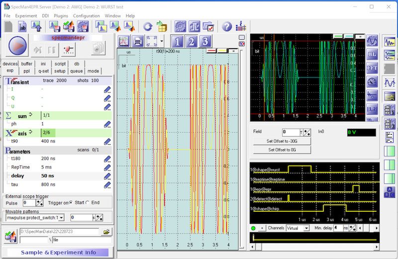
SpecMan4EPR - Connecting Spectrometers to People
The software features:
- Simple to use Graphical User Interface (GUI), so even non-expert users can setup complex experiments.
- Visualization of pulse sequences including all triggers.
- A powerful AWG engine for modern EPR experiments. The software comes with many different predefined pulse shapes (e.g. Chirp-Pulse, WURST-Pulse, etc.) but also allows for convenient upload of user specified pulse sequences.
- Flexibility to sweep variables. Almost every parameter can be defined as an axis in SpecMan4EPR and can be varied.
- Integrated magnetic field control for superconducting magnets.
2.2 - Installation
Software Installation
Typically, your Bridge12 EPR spectrometer comes pre-installed with SpecMan4EPR and the system is already configured depending on your needs and the available hardware. This includes all hardware drivers and any additional software that is required to operate the spectrometer.
SpecMan4EPR is not free and a licensed is required to run the software. This license file depends on the computer hardware and can not just simply transferred to a new computer. If you change the hardware, you may have to obtain a new license file to activate the software. To bet a new license file, please follow the instructions in the Troubleshooting Section
2.3 - Configuration
Typically, your EPR spectrometer will be delivered with a pre-configure version of SpecMan4EPR. Below, we provide a sample configuration. However, the exact values for certain parameters (e.g. COM port) may differ from system to system.
Device Configuration
To configure the different hardware component in SpecMan4EPR, open the Device Panel by clicking on the button labeled Configuration of devices (see button indicated by red box in figure below).
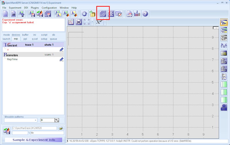
Once you click the button the Device Configuration window will open.
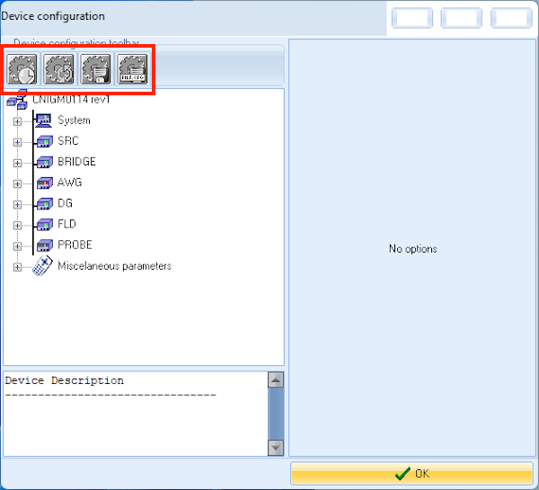
When you first open the Device Configuration window, you will be in Basic Access mode. In this mode, you can only view the parameters but you won’t be able to change any parameters or safe a new configuration. For this you need to access the Expert Mode. In the Basic Access mode, the safe and load buttons are greyed out.
To access the Expert Mode click Expert Access button to the top right of the window. You will be prompted with a password window. Simply acknowledge the password in the window by pressing the OK button. The Device Configuration window will change to Expert Mode (see figure below).
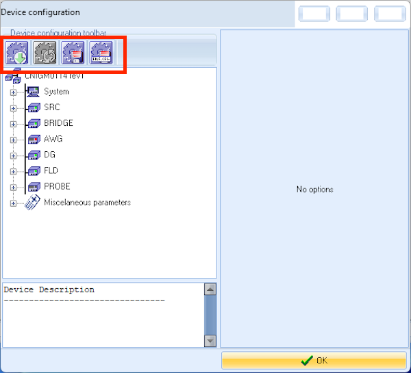
EPR Bridge
Bridge12 B12TXIF bridge controller and LabJackT7 (B12TXIF)
Driver version: 3.5
Interface 0: LabJack
Interface 1: Pixel controller
Name: BRIDGE
| Key | Value | Comment |
|---|---|---|
| Band | X-Band | Frequency band of the EPR bridge. |
| CGain1 | -27.142, 0.5714, 0, 0, 0, 0 | Polynomial coefficients (6th order) to adjust video amplifier gain. |
| CGain2 | -27.142, 0.5714,0 , 0, 0, 0 | Polynomial coeficients (6th order) to adjust video amplifier gain. |
| COMOptions1 | B115200M500 | Baud rate and timeout for DAQ device. Here the baud rate is set to 115200 and the timeout is set to 500 ms. These are default parameters for the Bridge12 X-IF and should not be changed. |
| CRvrLOAttn | -10, 0.667, 0, 0, 0, 0 | Polynomial coeficients (6th order) to adjust RCVR LO amplifier gain. |
| CVCA | -10, 4, 0, 0, 0, 0 | Polynomial coeeficients (6th order) to adjust RCVR amplifier gain. |
| DeviceID | CNIGM0114 | ID of DAQ device. Typically this is the Bridge12 project number. |
| Multithreaded1 | false | true or (false) Allows using of GPIB in multiple threads. Bridge12 typically does not use any GPIB devices. |
| Options1 | Leave blank | |
| ReadTime1 | 0 ms | none |
| Resource1 | COM3 | COM port of pixel controller. Use the Microsoft Device Manager (devmgr) to determine the correct port number. |
| TextReadProc1 | _A,A_,LFCR | Comma-separated: aA,Aa,_A,A_,LFCR |
| RextWriteProc1 | LF | none |
| WriteTime1 | 0 ms | none |
A sample configuration is shown below.
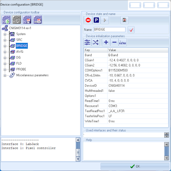
Microwave Source
Synth HD ver. 2.0 (SYNTHHD) Driver ver. 2.0
Name: SRC
| Key | Value | Comment |
|---|---|---|
| COMOptions | Leave blank | |
| Multithreaded1 | false | true or (false) Allows using of GPIB in multiple threads. Bridge12 typically does not use any GPIB devices. |
| Options | Leave blank | |
| ReadTime | 0 ms | Do not change. |
| Reference | R0F10 | Reference for microwave synthesizer. R(0/1/2) for External, Internal 27MHz, or Internal 10 MHz Reference. When using an external reference the frequency (in MHz) must be given. |
| Resource | COM4 | COM port of synthesizer. Use the Microsoft Device Manager (dvmgr) to determine the correct port number. |
| SourceOutputPow | 30 | Do not change. |
| TextReadProc1 | _A,A_,LFCR | Comma-separated: aA,Aa,_A,A_,LFCR |
| TextWriteProc | Leave blank | |
| WriteTime1 | 0 ms | none |
A sample configuration is shown below.
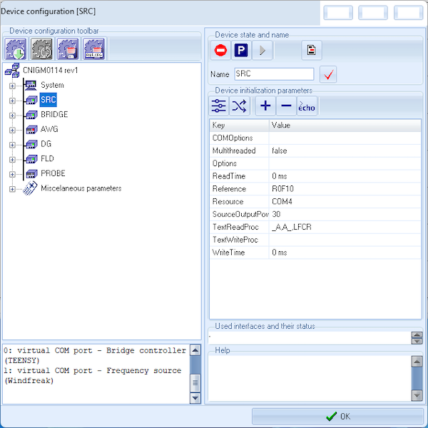
Digitizer
The configuration of the digitizer depends on the model and make you are using. Please contact support@bridge12.com for more information.
Arbitrary Waveform Generator (AWG)
The configuration of the arbitrary waveform generator (AWG) depends on the model and make you are using. Please contact support@bridge12.com for more information.
SpecMan4EPR Options
Please use the default SpecMan4EPR parameters for Directories and files. To access this go to Configuration and Select Options and expand the Directories and files menu.
| Parameter | Value |
|---|---|
| Configuration directory | C:\SpecMan4EPR\cfg |
| Template directory | C:\SpecMan4EPR\tpl |
| Data root directory | C:\SpecManDAta |
| Database root directory | C:\SpecManData |
| AWG pattern directory | C:\SpecMan\cfg\pattern |
| Directory with calibrations | \clb |
| Data buffer directory | C:\SpecManData\buffer |
| Data path format | <data root>\YY\YYMMDD |
| Station name | HOMEST |
| DLL paths | empty |
2.4 - Magnet Control
Two types of magnets are commonly used in EPR spectroscopy:
- H-Frame Electromagnets
- Superconducting Magnets
Most Bridge12 EPR spectrometers are equipped with a superconducting magnet. Both magnet types can be controlled through SpecMan4EPR.
2.4.1 - Superconducting Magnets
Important
The following instructions are specific to how the magnetic field is controlled through SpecMan4EPR. Instructions for cooling down the magnet can be found in the Magnet Section of the Systems Menu.
Warning
Superconducting magnets can produce extremely high magnetic fields. Avoid any metal objects around the magnet. Always operate around the magnet with care.
Please check with your local facility manager about safety procedures when working with superconducting magnets.
Overview
Superconducting magnets used in Bridge12 EPR spectrometers come with an integrated heater switch so the magnet can be operated in a driven-mode or in persistent mode. If the magnet switch is closed, the magnet is in persistent mode, similar to superconducting magnets. While the magnet will have the lowest drift rate in persistent mode, generating a very stable field, the field can not be swept/changed. To sweep the magnetic field, the heater has to be activated to open the switch.
A typical scenario to put the magnet in persisten mode at e.g. 5 T would look like this:
- Assuming the magnet is at 0 T activate the heater to open the (superconducting) switch. Wait until the heater reaches its target temperature (about 11 K).
- Ramp the field to the desired value, here 5 T. During ramping the field the magnet voltage will increase.
- Wait for the field to settle. This is indicated by the lowest voltage read by the power supply. When the magnet is at field, the voltage will never be 0 V, since this voltage also includes the voltage drop across the magnet leads.
- Deactivate the heater to close the switch. Wait for the heater to return to its base temperature.
- Ramp down the current in the magnet leads.
Warning
Contrary to what is done in NMR spectroscopy, do not disconnect the power supply from the magnet, once the magnet is set to persistent mode.
At the end of this procedure this the magnet is in a 5 T persistent field state and the drift will be very low. To change the field, first the magnet leads need to be ramped up to match the current in the magnet.
Warning
If the magnet is “parked” at a non-zero field and is in persistent mode, the current in the leads has to be ramped up to match the current in the magnet coil to avoid quenching or possible damage to the magnet.
The superconducting magnet power supply will not allow the user to activate the heater if the current in the leads does not match the current of the magnet coil.
If you encounter any problems please contact Bridge12 at support@bridge12.com.
2.4.1.1 - SpecMan Magnet Control GUI
The superconducting magnet can be completely controlled through the SpecMan4EPR software using the. From the SpecMan magnet GUI the user can activate the heater switches, move/sweep the magnet field, and can put the magnet in persistent mode.
Launching the Magnet GUI
To launch the magnet GUI:
- Go to the DDI menu
- Select Set Field from, FLD from the menu. This will open a separate window with all magnet controls.
The following window will appear:
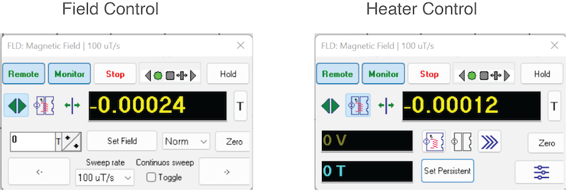
The magnet control window has three different buttons to select the functionality:
- Heater Control: Click this button to access the heater controls to enable/disable the heater switch (see figure above, left).
- Field Control: Click this button to access the field controls to change/set the magnetic field strength (see figure above, right).
- Polarity Control: Click this button to change the polarity of the magnetic field (currently not used) (not shown/used).
2.4.1.2 - Heater Control
To change the magnetic field first the superconducting heater needs to be activated. This will connect the magnet power supply to the main coil and will allow the user to increase or decrease the current in the main coil and therefore moving the magnetic field.
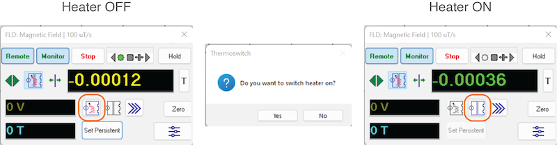
The value of the magnetic field is shown in two different colors, depending if the heater switch is activated or not:
- Yellow : The heater switch is off. If the field is at a value of 0 T, the main coil is completely discharged. If the value is not 0 T it means the magnet is in persistent mode, and the field is “parked” at that value. Before activating the switch, the current in the magnet leads not to ramped back to the persistent mode value (see figure above, left).
- Green : The heater switch is activated (on) and the field can be moved (see figure above right).
Warning
The switch in the superconducting magnet is thermally activated. When activating the heater (switching the heater on) the user should wait for 10-20 seconds until the switch is fully opened. To be sure the switch is fully openend, the user can check the heater switch temperature in the logging GUI.
Operating the Switch
Opening the Switch at 0 T
To open the superconducting switch:
- If the magnetic field is at a value of 0 T, click the icon to open the switch in the magnet GUI (see figure above, left).
- Confirm that you want to open the switch by clicking Yes in the dialog box.
- Wait for 10 - 20 seconds for the switch to fully open.
Opening the Switch when Magnetic Field is not at 0 T
To open the superconducting switch:
- Enter the value of the persistent field to charge the current in the leads to match the current when the switch was closed.
- Wait for the power supply to reach the field.
- Click the icon to open the switch in the magnet GUI (see figure above, left).
- Confirm that you want to open the switch by clicking Yes in the dialog box.
- Wait for 10 - 20 seconds for the switch to fully open.
Closing the Switch
To close the superconducting switch:
- Click the icon to close the switch in the magnet GUI (see figure above, right).
- Wait about 10 - 20 seconds for the switch to close
2.4.1.3 - Operating the Magnet
Depending on the type of experiment the magnet field is either:
- Moving For example in a echo-detected field-sweep experiment. Here, the field is swept while recording the echo intensity.
- Static For example in a DEER/PELDOR experiment. These type of experiments are performed at a static magnetic field value. If the user does not change the field for a long time (e.g. an overnight experiment), it is recommended to put the magnet in persistent mode.
Typically, when switching on the spectrometer, the user would set a field value close the start value. This is not strictly required but will speed up operations when the field is moved a lot during an experiment session.
Once an initial value is set the field is entirely controled by SpecMan4EPR.
Setting an Initial Field Value
To prepare for an experiment:
- Open the SpecMan4EPR Magnetic Field GUI.
- Click on the heater control icon.
- Activate the superconducting heater switch. After you clicked the icon to activate the switch wait for about 10 - 20 s for the switch to completely open.
- Click the icon to control the magnetic field.
- Enter the desired value for the magnetic field and press the ENTER key.
- Wait for the magnet power supply to reach the desired magnetic field value.
- (Optional) If the EPR experiments are performed at a static magnetic field, close the superconducting magnet switch to put the magnet in persistent mode. Enter a value of 0 T for the magnetic field to ramp down the current in the magnet leads.
Ramping Down the Magnet
It is completely fine to leave the magnet at field, if the spectrometer is not used for a short time. However, if the spectrometer is not used for a while, the magnetic field should be discharged. To ramp down the magnet:
- (Optional) If the magnet is in persistent mode:
- Enter the field value, matching the magnetic field value of the magnet and hit the ENTER key.
- Wait for the power supply to reach the value.
- Open the superconducting magnet switch. After you clicked the icon to activate the switch wait for about 10 - 20 s for the switch to completely open.
- Enter a value of 0 T for the magnetic field strength and hit the ENTER key.
- Wait for the magnet to reach a field of 0 T.
- Once the magnet reached 0 T, close the superconducting magnet switch.
Information
Unless the spectrometer is not used for several days, the Helium compressor will be constantly running and is not turned off, when the spectrometer is switched off. Keep in mind, it takes about 24 hrs to cool down the magnet from room temperature.
Changing the Ramp Rate
When sweeping or changing the magnetic field, the rate, at which the magnetic field is changed, can not exceed a specific value. This value for the sweep rate is given by the magnet manufacturer. It is common for superconducting magnets to have different sweep rates for different field value regimes.
2.5 - Troubleshooting
2.5.1 - SpecMan4EPR
Software Installation
Debugging
Debugging the LabJack Interface
Software Installation
Re-Installing SpecMan4EPR on new Hardware
In case have to re-install SpecMan4EPR on a new computer, follow these steps (assuming you saved a previous copy of SpecMan4EPR):
- Start by creating two folders in the main directory (C:).
- C:\SpecMan4EPR
- C:\SpecManData
- Copy the SpecMan4EPR application (SpecMan4EPR.exe) into the application directory (C:\SpecMan4EPR)
- Inside the SpecMan4EPR folder create three subfolders:
- cfg - to store configuration files
- pattern - to store pattern files
- tpl - to store pulse program templates
- Double click the SpecMan4EPR icon to start the application. Since no license is installed, SpecMan4EPR will create a LIF File. To obtain a license please send this file to support@bridge12.com and include any additional information about your spectrometer (e.g. serial number)
- You will receive a license file (Specman4EPR.nlic). Move this file into the SpecMan4EPR directory. This will activate your software license and you will be able to use SpecMan4EPR.
Debugging
Serial Communication
Serial communication in SpecMan4EPR is most conveniently debugged in the built-in script editor.
LabJack DAQ Interface
To debug communication with the LabJack interface and to enable the verbose mode for the LabJack interface follow these steps:
- In SpecMan4EPR to the the Script tab
- Select the LABJACK interface from the dropdown menu
- Select S00
- From the command dropdown menu select .echo
- Enter 1 in the empty text box
- Hit ENTER.
Once the verbose mode is enabled, open the Log Window by clicking the View log window in the toolbar to the right. For clarity, you can clear the log by right clicking with the mouse into the window and click Clean Log. This will clear all old messages.
2.5.2 - Magnet
Magnet Control
Recovering after Magnet Quench
Recovering after Magnet Quench
A magnet quench can occur for several reasons, such as sudden loss of electricity, or the cooling water supply shuts down. If the helium compressor shuts off while the magnet coils are charged, or are in persisten mode, the user has about 8 minutes left until the magnet coils have reached about 8 K and the magnet will quench. However, in contrast to a wet magnet, this is rather uneventful. The temperatures of all sensors will suddenly increase. Once electricity (or cooling water) is back, the helium compressor will restart automatically and the magnet will be cooled. If the compressor doesn’t restart automatically, it has to be done manually.
Once the magnet has reached its base temperature it is again safe to operate the system. The temperatures can be observed either directly on the temperature monitor or through the systems logger. Typical temperatures are:
| Sensor Name | Typical Temperature (K) |
|---|---|
| Cryo Head (1st Stage) | ~ 37 K |
| Cryo Head (2nd Stage) | ~ 3 K |
| Magnet Coil (LHS, RHS) | ~ 3 K |
| Heater Switch | ~ 5.5 K |
To energize the magnet again follow these steps:
- Make sure the helium compressor is running and that the magnet has reached its base temperatures (see table above).
- The power supply may show the message HEATER switched off at XX.XXX Amps. This indicates, the magnet was in persistent mode when the quench occurred. However, the user can safely ignore this message. To clear this message:
- If the power supply is in remote control mode, take the power supply back into local front panel operation mode by pressing the button labeled REMOTE.
- Press the HEATER button to activate the switch (the LED light will come on). Wait for a few seconds.
- Press the HEATER button again to switch the heater off.
Alternatively, the user can just restart SpecMan4EPR and start using the magnet.
3 - System Monitor - pyB12Logger
The pyB12Logger is a general purpose logging software to log the status of different devices that are connected to the spectrometer (e.g. cryo-compressor, temperature controllers, …). The software is distributed as a Python package.
When the software is started for the first time, it will automatically create some configuration files and directories on the hard disc to store the log files.
The log files are written as a comma separated value (csv) file.
The Python package has two components:
- pyB12logger This is he logger software, which will run in the background. Typically, it is automatically started when the computer starts up.
- pyB12monitor This is a program to plot the logged data. The monitor can be used to plot real-time data or historical data from the log files.
Requirements
- Operating System: Windows 10 (or higher)
- Python, version > 3.6
Using the Logger
Starting the Logger
Typically, the logger is started automatically for example, after the computer re-boots. To start the logger manually follow these steps:
- Open a command prompt window by typing
cmdinto the window search bar. - At the command prompt type
pyB12Loggerand hit the return key.
After hitting the return key a status message will inform the user whether the logger is already running, or if it has been started (see screen shot below).
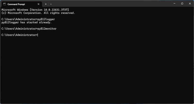
The general format it the command is:
pyB12logger [-h] [-desktop {True,False}] [-startup {True,False}] [-debug {True,False}] [{start,stop}]
| Arguments/Options | Description |
|---|---|
| {start,stop} | Start or stop the pyB12logger. If no argument is given, the command will start the logger |
| -h, –help | Show help message |
| -desktop {True,False} | Create a desktop icon for the software |
| -startup {True,False} | Enable or disable the starting the pyB12logger when the computer boots |
| -debug {True,False} | Start the pyB12logger with console window |
Starting the Monitor
The pyB12monitor is used to either plot historical data or the real-time data. To type start the monitor:
- Open a command prompt window by typing
cmdinto the window search bar. - At the command prompt type
pyB12monitorand hit the return key.
The pyB12monitor will start.
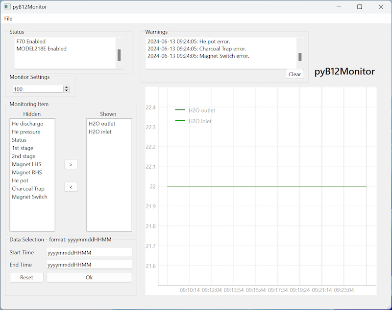
| Name | Description |
|---|---|
| Status | Status of the devices |
| Warnings | Warning messages are shown here. Warnings are based on the min, max, static values given in the configuration file |
| Window Length | Number of data points shown in the graph |
| Hidden | List of variables that are logged |
| Shown | List of variable that are shown in the plot |
| Arrows | Move variables from Hidden to Shown and vice versa |
| Start Time & End Time | Optional parameters. These values can be used to select a certain time range to be plotted. Click OK to confirm the time range. Click Reset to return to the real-time view |
All settings are automatically saved.
Configuring the Logger
- Data logs are located at C://Users/Public/B12TLOG
- The typical file size is 100 kB. This value can be adjusted by the user in the configuration file.
- The configuration file is located at C://User/Public/B12TLOG_Config/config.cfg
The first section of the config file is the [SETTINGS] section. It contains information about the logging interval (given in s), the location of the log files, and the maximum file size.
[SETTINGS]
log_interval = 10
log_folder_location   = C:/Users/Public/
save_file_size_kb   = 100
This section is followed by individual sections for different instruments that are connected to the logger.
[F70]
device_status = True
address = ASRL11::INSTR
termination = CR
id_command = $ID1D629
index = 1
helium_discharge_temperature  = $TE140B8, alias = He discharge
water_outlet_temperature      = $TE241F8, alias = H2O outlet, min = 10, max = 35
water_inlet_temperature       = $TE38139, alias = H2O inlet, min = 10, max = 35
compressor_pressure           = $PR171F6, alias = He pressure
status                        = $STA3504, alias = Status, static = 301
For more information about how to configure the pyB12logger, please contact Bridge12 at support@bridge12.com.
Installation
The software comes installed and pre-configured with the spectrometer. If you need to re-install the software please contact us at support@bridge12.com.
4 - DNPLab
DNPLab is an object-oriented Open Source Python-based package for importing, processing, and analyzing data recorded in a Dynamic Nuclear Polarization (DNP) experiment. The aim of the project is to provide a free, turn-key python-based processing package DNP-NMR data.
DNPLab is a collaborative project created by:
- Bridge12 Magnetic Resonance LLC
- The Han Lab at Northwestern University
- The Franck Lab at Syracuse University
DNPLab is distributed free of charge under the MIT License.
For more information:
- Visit the Online Documentation of DNPLab
- Follow us on Twitter
- Check out the DNPLab GitHub Repository
- Please report all issues on the DNPLab GitHub Issue Tracker