Welcome to the online documentation of our systems for EPR, NMR and DNP spectroscopy. Bridge12 does not distribute paper manuals with the equipment to ensure our documentation is always up to date. If you have questions, or suggestions for edits please contact us at info@bridge12.com.
Important
Please read the documentation for you product carefully to avoid any damages to the Bridge12 system.
1 - Spectrometers
Systems for EPR, NMR, and DNP Spectroscopy
1.1 - X-Band IF
Bridge12 X-Band IF System for Pulse EPR Spectroscopy
The Bridge12 X-Band IF system is at the heart of all Bridge12 EPR spectrometers. The system is highly modular. For X-Band EPR spectroscopy only a high-power microwave amplifier, digitizer and AWG is required.
The system can be completely controlled using SpecMan4EPR.
1.1.1 - Bridge12 X-IF System Overview
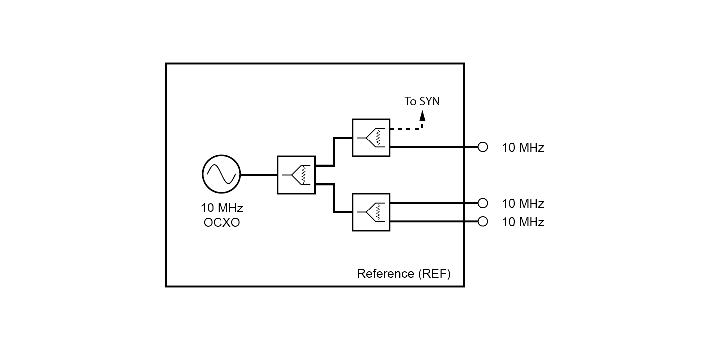
Bridge12 X-IF System Overview
Bridge12 X-IF Overview Schematic
The Bridge12 X-IF system consists of four different sub-systems:
Pulse Forming Unit (PFU): - IQ mixer based pulse forming unit.
Receiver Unit (RCVR): - IQ mixer based receiver unit with video amplifiers.
A schematic of the entire system is shown in the figure above. Most of the connections of the individual sub-systems are routed to the back panel of the system (shown as circles) to provide the user maximum flexibility. Only a few connections are made internally and cannot changed by the user (dashed lines). In the following section a brief description of each sub-systems is given.
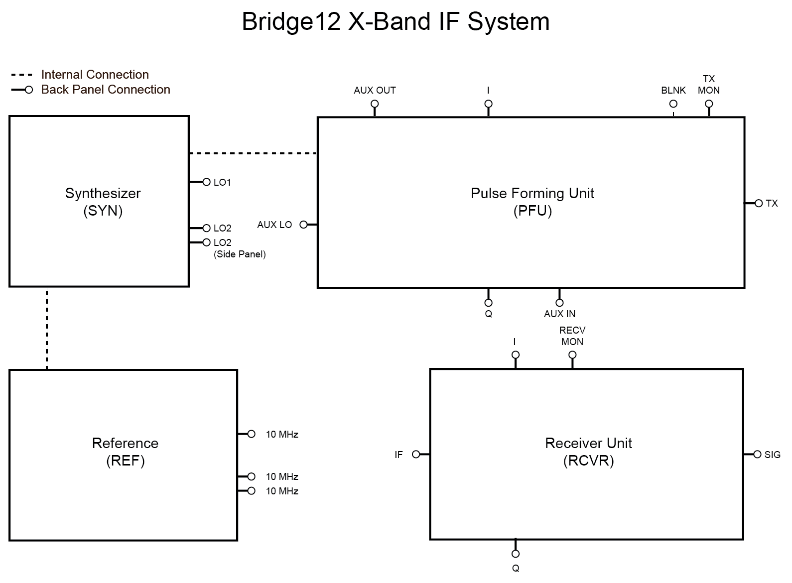
Synthesizer (SYN)
The Bridge12 X-IF system has an integrated microwave synthesizer with two independent channels, LO1 and LO2. The signal of both channels is split into two signal paths. Both signals (LO1 and LO2) are available on the back panel. LO1 is also connected internally to the input of the Pulse Forming Unit (PFU). LO2 is also available on the side panel of the X-IF system, below the signal (SIG) input.
Both microwave synthesizers are locked to the internal 10 MHz reference clock. By default both channels are phase locked to each other. This can be changed through the software.
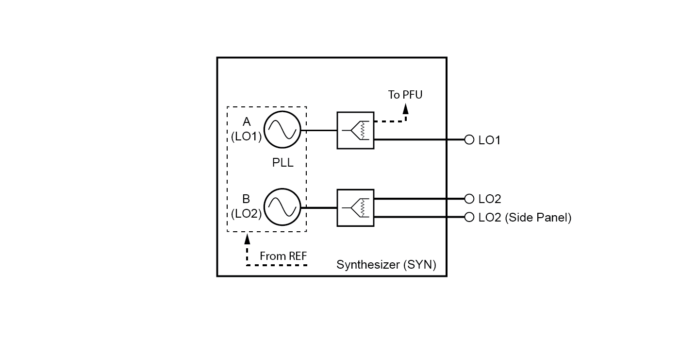
Reference (REF)
The Bridge12 X-IF system has an integrated oven-stabilized 10 MHz reference clock. Three 10 MHz outputs of the reference clock are available on the backpanel. This can be used to sync other devices such as an AWG or Digitizer. One channel of the clock is internally connected to the synthesizer for phase locking.
Note
The output level of all 10 MHz reference back panel connectors is 2 Vpp into 50 Ω.
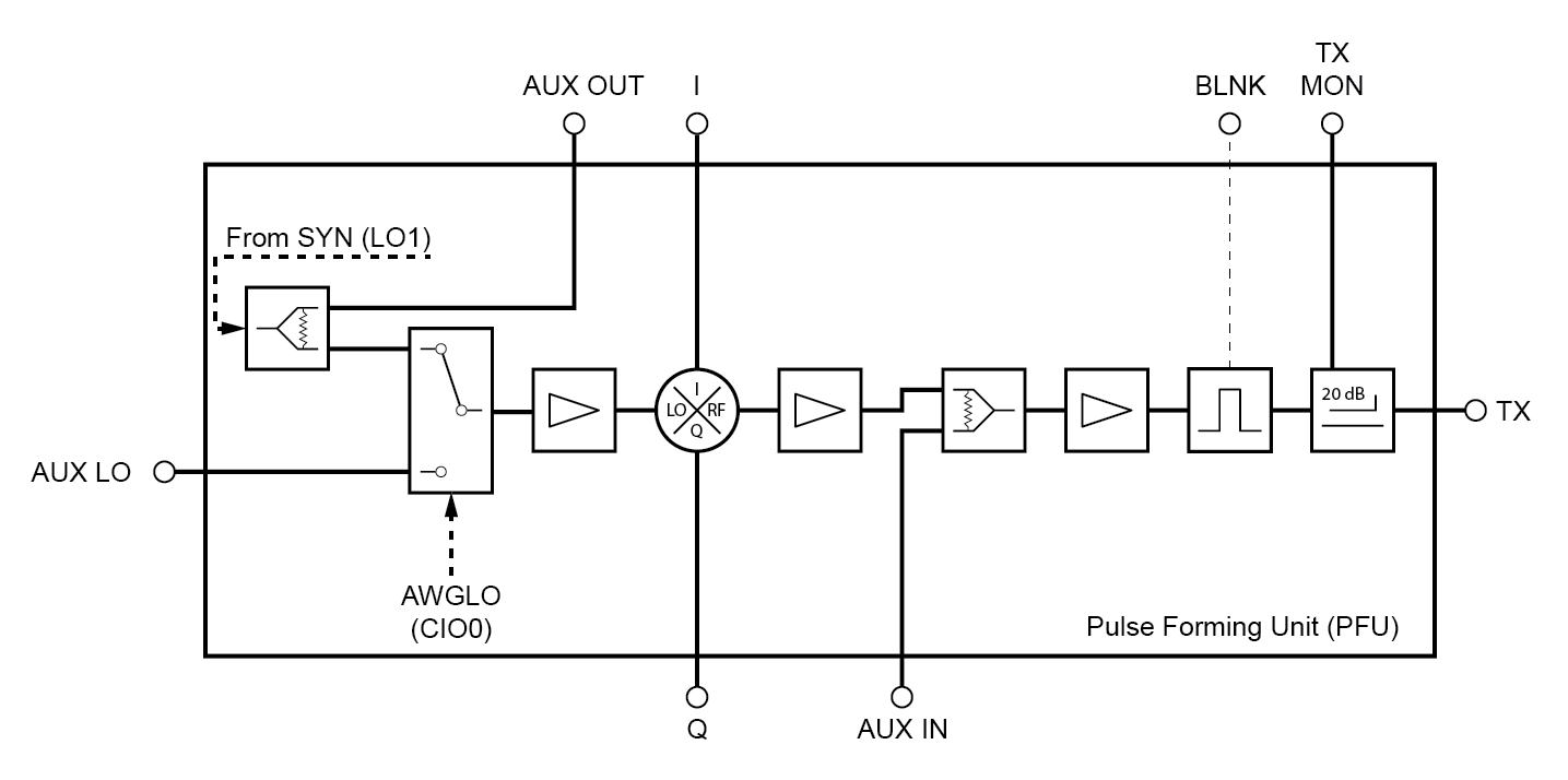
Pulse Forming Unit (PFU)
Pulses in the X-IF system are created by the Pulse Forming Unit (PFU). At the heart of the PFU is an I/Q mixer. Both channels, I and Q would normally be driven by an AWG. However, to create rectangular pulses at the LO1 frequency, these channels can also be driven by rectangular pulses created by a pulse programmer.
Internally, the LO of the IQ mixer is connected to LO1 of the synthesizer. However, a different LO signal can be supplied through the back panel connector AUX LO. If a rectangular pulse is applied to the I and Q channels, the pulse frequency will be identical to LO1. If a waveform is supplied (e.g. rectangular pulse at f(AWG) = 250 MHz) the output frequency at TX will be LO1 + f(AWG).
The output signal of the IQ mixer (RF) is amplified and sent to the TX back panel connector. The PFU has a blanking switch. The BLNK gate should be connected to a pulse programmer (or a marker/channel of the AWG if available). The gate is active HIGH. In between pulses, this gate should be LOW to minimize any LO bleed-through.
The microwave pulses generated by the PFU can be directly monitored on the TX MON backpanel connector.
An auxillary LO signal can be supplied to the IQ mixer by connecting the AUX LO input to for example the LO2or an external synthesizer. The rise/fall time for this switch is about 10 ns. This can be used for example to create a non-coherent microwave pump pulse in a DEER experiment. Alternatively, an additional signal can be supplied to the AUX IN connector.
PFU Control Signals
Component
SpecMan Control Signal
LabJack Control Signal
Function
AUX LO Switch
AWGLO
CIO0
Select LO signal for IQ mixer
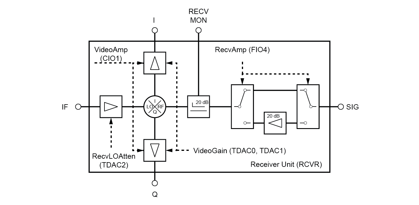
Receiver Unit (RCVR)
The Bridge12 X-IF is equipped with a IQ mixer based Receiver Unit. The signal from the probe is connected to the SIG side panel connector.
Note
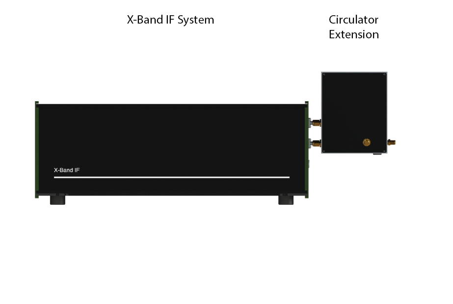
To give the user the most flexibility what type of probe to connect to the system, the X-IF system does not have an integrated low-noise amplifier (LNA) or circulator. For X-Band operation an external circulator/LNA module is available that can be connected to the X-IF system. Otherwise, the circulator and LNA is part of the frequency extension.
The input signal can be further amplified using an internal amplifier with about 20 dB gain. The receive signal can be monitored on the RECV MON back panel connector. This signal is sent to the RF port of the IQ mixer. The LO signal for the IQ mixer is supplied to the IF back panel connector. For X-Band operation, IF is typically connected to LO1, the same signal supplied to the PFU.
Note
If the IF port is connected to the LO1 port and an AWG is used to generated pulses at an offset frequency of f(AWG), the detected EPR signal is at this frequency. The signal can then be digitally demodulated and filtered.
The down-converted signal is further amplified by a pair of video amplifiers. The gain of the video amplifiers is variable, and the video amplifiers can also be bypassed. The down-converted EPR signal is available at the I and Q back panel connectors. This signal can be either sent to a digitizer or lock-in amplifier for detection.
RCVR Control Signals
These signals
Component
SpecMan Control Signal
LabJack Control Signal
Function
Microwave Amplifier
RecvAmp
FIO4
Pull High to enable the microwave signal amplifier
Video Amplifiers
VideoAmp
CIO1
Pull HIGH to enable the video amplifiers
Video Amplifier Gain
VideoGain
TDAC0, TDAC1
Variable gain control of the video amplifiers
LO Amplifier
RecvLOAtten
TDAC2
Receiver LO amplifier to set LO level of IQ mixer
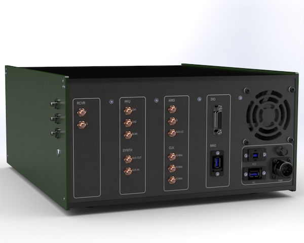
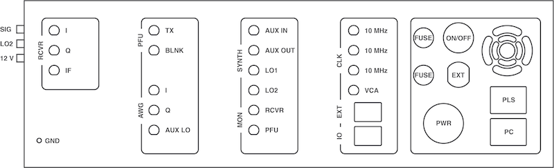
1.1.2 - X-Band IF Backpanel Connections
Backpanel connections of the X-Band IF system.
Below, please find a list and description of the backpanel connectors of the X-Band IF system. Please refer to the figure below for the location of connections.
Warning
Whether a connector is used for an input or output signal is labeled in the table below. Please make sure the user makes the correct connections. Wrong connections can lead to permanent damages of the system.
RF Connections
Please refer to the table below for a description of the back panel connectors of the X-Band IF system. The function (I/O - input/output) of the connector is indicated in the second column.
Information
Make sure all connections to the back panel connectors are properly tighten. SMA connections should be tightened using a torque wrench (recommended torque 10 Nm).
Side Panel
Connector
I/O
Type
Description
SIG
I
SMA
Input signal for the receiver.
LO2
O
SMA
LO2 output of the microwave synthesizer (channel B)
Back Panel
Receiver (RCVR)
Connector
I/O
Type
Description
RCVR I
O
SMA
I channel of the quadrature receiver channel. This is typically referred to as the real signal of the detected EPR signal.
RCVR Q
O
SMA
Q channel of the quadrature receiver channel. This is typically referred to as the imaginary signal of the detected EPR signal.
RCVR IF
I
SMA
IF input of the RCVR. For X-Band operation, this should be connected to the LO1 output of the microwave synthesizer (channel A). Suggested Cable
Pulse Forming Unit (PFU) and AWG Input
Connector
I/O
Type
Description
PFU TX
O
SMA
Output of the PFU. This signal is typically routed to the high-power amplifier or the active multiplier chain (AMC) in high-field/high-frequency EPR spectrometers.
PFU BLNK
I
SMA
Blanking gate of the PFU. TTL logic. Active high. This signal has to be connected to the pulse programmer.
AWG I
I
SMA
I channel input of the PFU. This signal needs to be connected to the output channel of the AWG.
AWG Q
I
SMA
Q Channel input of the PFU. This signal needs to be connected to the output channel of the AWG.
AWG AUX
I
SMA
Auxillary input of the IQ mixer LO channel.
Synthesizer and Monitors
Connector
I/O
Type
Description
AUX IN
I
SMA
Auxillary microwave signal input. This signal is combined with the microwave signal generated by the IQ mixer of the PFU and allows the user to inject an additional, user-created microwave signal.
AUX OUT
O
SMA
LO signal of the LO input for the IQ mixer of the PFU. This signal is similar to LO1.
LO1
O
SMA
LO1 signal of the X-Band IF system (channel A of the synthesizer).
LO2
O
SMA
LO2 signal of the X-Band IF system (channel B of the synthesizer).
0 - 5 V DC signal. The output level of this signal can be controlled through the software. This signal is typically used for the Voltage Controlled Attenuator (VCA) of a high-frequency AMC.
12 V output. This supply voltage can be used to power up external equipment. Do not exceed 200 mA. Mating Connector
Other Connectors
Connector
I/O
Type
Description
EXT PWR
O
M12
Power supply e.g. for a frequency extension. Available voltages: -12 V, -5 V, 5 V, 12 V, 15 V
PWR
I
Amphenol
Power inlet for the X-Band IF system. Please only use the power supply supplied with the system to avoid permanent damages.
PLS
I/O
USB
USB connection from the X-Band IF to the pulse programmer. This USB port is connected to the internal USB hub of the X-Band IF system.
PC
I/O
USB
USB connection to remote PC.
GND
n/a
STUD
A ground (GND) post is located in the lower left corner of the back panel.
Warning
Only use the power adapter that came with the X-Band IF system to power up the instrument.
Failure to use the correct power adapter can lead to permanent damage of the system.
If you are unsure about the power adapter, please contact Bridge12 at support@bridge12.com
1.1.3 - Digital Demodulation
How to use digital demodulation with the X-Band IF system.
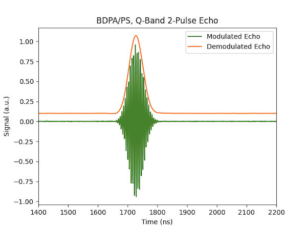
The Bridge12 X-Band IF system supports digital demodulation. Digital demodulation allows for easy removal of baseline artifacts and will result in a much cleaner signal detection. Instead of down-converting the EPR signal to DC level, the LO frequency is slightly offset and the signal is detected at a frequency of e.g. 200 MHz. The exact frequency depends on the sampling rate and input bandwidth of the digitizer (or oscilloscope).
Information
Digital demodulation is highly recommended for the X-Band IF system. Even an offset of just 20 MHz will greatly remove many artifacts from the baseline.
The example below shows a digitally demodulated signal of a 2-pulse Hahn echo of a sample of BDPA in polystyrene, recorded at Q-band frequencies.
We recommend using an intermediate frequency of about half the bandwidth of the digitizer. For example, if the digitizer has an input bandwidth of 400 MHz, we recommend to choose an intermediate frequency of 200 MHz.
Digital Demodulation (Recommended Operation)
To acquire the EPR signal at a This offset can be achieved in two ways:
1. Offsetting the AWG Frequency
The simplest way to use digital demodulation is by offsetting the frequency for the AWG generated microwave pulses. Instead of generating a rectangular pulse at DC level, the user can create a pulse at a frequency of e.g. 200 MHz. To make sure the frequency of the microwave pulse is within the bandwidth of the resonator, the microwave frequency needs to be lowered by the same amount. For example, to generate a microwave pulse at 9.8 GHz with an offset of 200 MHz:
Set the LO1 frequency of the synthesizer to 9.6 GHz (9.8 GHz - 0.2 GHz)
Set the AWG frequency to 200 MHz
Set the demodulation frequency in SpecMan4EPR to -200 MHz.
2. Offsetting the Receiver Frequency
If pulses are not created by an AWG but for example by a pulse generator, digital demodulation can still be used. However, in this case, both microwave synthesizers, LO1 and LO2, have to be utilized.
To use digital demodulation with DC pulses follow these steps:
Connect the RCVR IF to the LO2 output.
Set the LO1 frequency on-resonant with the resonator frequency, e.g. 9.6 GHz.
Set the LO2 frequency to 9.4 GHz. That way the echo signal has to be demodulated using a frequency of 200 MHz (9.6 GHz - 9.4 GHz = 0.2 GHz).
Demodulating the Signal (Demodulating the Signal)
Once the signal is digitized it has to be digitally demodulated.
In SpecMan4EPR
Demodulating the EPR signal in SpecMan4EPR is very straight forward and simple. Simply make sure the Demodulation Frequency is set to the correct value and the spectrum is automatically demodulated when the data is acquired.
Manually
If the X-Band IF is used manually, demodulation must be performed by the user during post-processing of the EPR data. This can be conveniently done by using the demodulate function in DNPLab.
DC Detection
To down-convert the EPR signal to DC level, connect the LO1 output of the synthesizer to the IF input of the receiver and make sure the frequency offset for the AWG pulses is set to 0 MHz.
1.1.4 - Circulator Attachment
Connecting the circulator attachment to the the X-Band IF system.
The Bridge12 X-Band IF does not have an integrated circulator/pre-amplifier, instead an attachment is connected to the side panel of the X-IF system. This attachment will look slightly different for different frequency bands (X-Band, Q-Band, etc.). For some other frequency bands such as S-Band, or W-Band, the circulator is integrated into the frequency extension.
X-Band Circulator
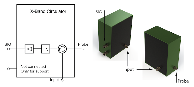
The X-Band circulator attachment is directly connected to the side panel of the X-IF system (see figure above) and is held by two SMA connections. A schematic of the circulator attachment is shown in the figure below.
The circulator attachment has three connectors:
Input: This connector needs to be connected either to the output of the high-power microwave amplifier for pulsed experiments, or to the TX or the LO1 (LO2) output of the X-IF (back panel connector).
Probe: The EPR probe is connected to this connector.
SIG: This is the signal output which is connected to the side panel of the X-IF system. The SMA connector below is only for support and is internally terminated with 50 Ω.
1.1.5 - Example Configurations
Example configurations for different frequency bands.
The Bridge12 X-Band IF system can be used to operate EPR spectrometers from S-Band (2 GHz) to the millimeter regime (> 400 GHz).
Below, please find example configuration for different operating frequencies.
1.1.5.1 - Example: Pulsed X-Band Operation
Example configuration for pulsed X-Band EPR spectroscopy.
A typical configuration of the X-Band IF system for pulsed X-Band spectroscopy is shown in the figure below. Connections that are not required are greyed out.
Connector
Description
RCVR IF to LO1
Connect a microwave cable between the LO1 synthesizer output and the RCVR IF input. This has to be a microwave cable, able to carry frequencies up to 10 GHz (Suggested Cable). This is the default configuration when using digital demodulation and offsetting the pulse frequency using the AWG.
RCVR I RCVR Q
Connect the RCVR I and RCVR Q channel to the digitizer or oscilloscope. The EPR signal will appear here.
AWG I AWG Q
Connect the AWG I and AWG Q connectors to the arbitrary waveform generator. Alternatively, these channels can also be connected directly to the output of a pulse programmer to generate rectangular pulses at the LO1 frequency. If you have questions about these mode, please contact Bridge12 at support@bridge12.com.
PFU TX
This is the output of the X-Band IF system. Connect this connector to the input of the high-power pulse amplifier. Depending on the type of the amplifier an additional pulse blanking gate is required as a channel of the pulse programmer.
PFU BLNK
Blanking gate of the PFU. This is not the amplifier blanking gate. This gate is active high and needs to be high to be able to transmit microwave pulses.
10 MHz CLK
Connect the system clock to each, the digitizer and the AWG. That way, the X-Band IF system provides the master clock to synchronize all other instruments. The X-Band IF master clock runs at 10 MHz. In cases when the AWG clock is higher, the user may want to synchronize the system to the AWG clock to minimize pulse jitter.
1.1.6 - Manual Operation of the X-Band IF
Required software to install to manually operate the X-Band IF system.
To manually operate the X-Band IF system please install the following software:
Digital/Analog Controls: Please download Kippling distributed by LabJack.
Once these two software packages are installed, the X-Band IF system can be completely remote controlled.
1.1.6.1 - Controlling the X-Band IF Synthesizer
How to control the X-Band IF microwave synthesizer manually
Please make sure the control software for the synthesizer is installed. If you haven’t done so, you can download it here.
1.1.6.2 - DAQ Control
How to control the analog and digital lines of the X-Band IF system manually.
Please make sure the control software for the DAQ interface is installed. If you haven’t done so, you can download it here.
Connecting to the DAQ Interface
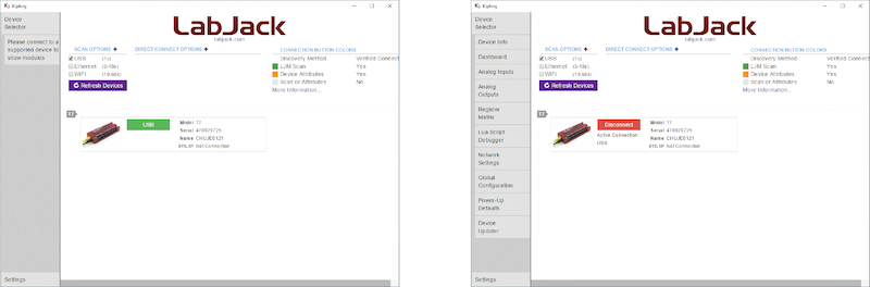
To connect to the DAQ interface follow these steps:
Make sure the X-Band IF USB interface is connected to the host computer.
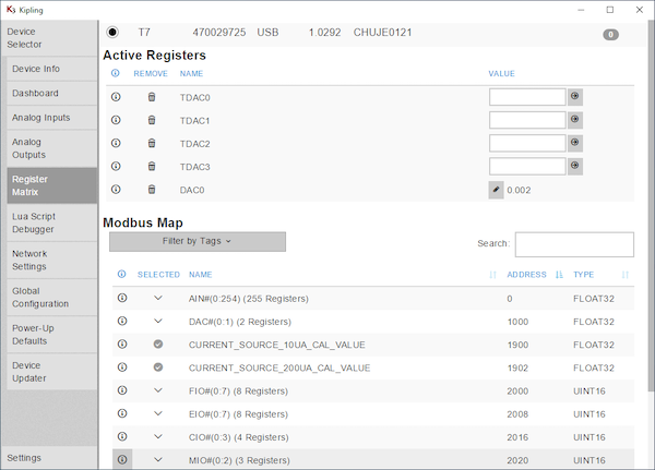
Start Kipling
In the GUI click the green USB button (see figure above, left). The USB button will turn red, indicating that Kipling is connected to the DAQ interface (see figure above, right).
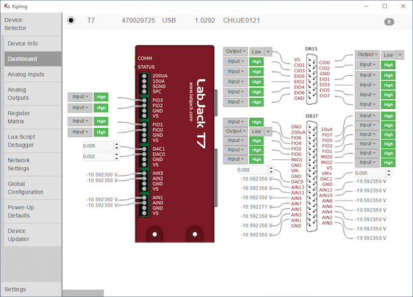
Digital Input/Output Control
To control the digital input/output lines click on the menu item Dashboard (see figure above). Each of the lines can be configured as an input or output by selecting the control from the drop-down menu. If the line is configured as an input the indicator to the left will show whether the line is logic high or low. If the line is configured as an output, the status can be changed by selecting the desired status from the drop-down menu.
Below is a list of the different digital channels used by the X-Band IF system.
Pulse Forming Unit (PFU)
Bit Name
Function
CIO0
AWG LO select for PFU. 0 - Internal synthesizer (LO1), 1 - AUX LO, auxillary LO input on back panel
Receiver (RCVR)
Bit Name
Function
CIO1
Enable/Disable video amplifiers. 0 - disabled, 1 - enabled
FIO4
Microwave signal amplifier, 0 - disabled, 1 - enabled +20 dB gain
Analog Output Control
The value of the various analog outputs can be controlled from the Register Matrix panel. The values for TDAC0 - TDAC3 can be set between -10 and +10 V, with a resolution of 16 bit.
Below is a list of the different analog channels used by the X-Band IF system.
Receiver
Bit Name
Function
TDAC0
Video amplifier gain control (I channel), value from -10 to 10 V, -10 V - 30 dB gain, 10 V - 65 dB gain
TDAC1
Video amplifier gain control (Q channel), value from -10 to 10 V, -10 V - 30 dB gain, 10 V - 65 dB gain
TDAC2
LO level receiver, value from -10 to 10 V, -10 V - 0 attenuation, full power on LO of IQ mixer (RCVR), 10 V - 30 dB attenuation, lowest power on LO of IQ mixer (RCVR)
Miscellaneous Other Controls
The X-Band IF system has several spare digital and analog input and output lines connected to the IO and EXT connector located on the back panel. These lines can be configured by the user.
Note
For most sub-D connectors the pin number is either printed on the front either at the pin (male connector) or the receptacle (female connector).
EXT Connector (9 pin sub-D, back panel)
The external connector is most commonly used to control an extension to the X-IF system, such as a frequency extension.
All lines are configured as outputs in SpecMan.
Pin Number sub-D
Bit Name (LabJack)
SpecMan Variable
Function
Reserved For
1
EIO0
Ext1
DAQ bit EIO0, can be configured as input and output, TTL level
2
EIO2
Ext3
DAQ bit EIO2, can be configured as input and output, TTL level
3
EIO4
Ext5
DAQ bit EIO4, can be configured as input and output, TTL level
4
EIO6
Ext6
DAQ bit EIO6, can be configured as input and output, TTL level
5
GND
n/a
System GND
6
EIO1
Ext2
DAQ bit EIO1, can be configured as input and output, TTL level
7
EIO3
Ext4
DAQ bit EIO3, can be configured as input and output, TTL level
8
EIO5
Ext6
DAQ bit EIO5, can be configured as input and output, TTL level
9
EIO7
Ext8
DAQ bit EIO7, can be configured as input and output, TTL level
IO Connector (9 pin sub-D, back panel)
Pin Number sub-D
Bit Name (LabJack)
SpecMan Variable
Function
Reserved For (SpecMan)
1
MIO0
IO1
DAQ bit MIO 0, can be configured as input and output (TTL level)
Enable/disable tune mode
2
MIO2
IO3
DAQ bit MIO 2, can be configured as input and output (TTL level)
3
DAC1
DAC1
DAQ bit DAC 1. This is an analog output. The value can be changed between 0 and 5 V. The output is controlled from the Dashboard menu
4
AIN1
DAQ bit AIN1, analog input range ±10V, ±1V, ±0.1V and ±0.01V
5
GND
n/a
System GND
6
MIO1
IO2
DAQ bit MIO 1, can be configured as input and output (TTL level)
Enable/disable external high-power amplifier
7
TDAC3
TDAC 3, values (set in software) -10 to 10 V, output is 0 to 10 V, 14 bit resolution
8
AIN0
DAQ bit AIN0, analog input range ±10V, ±1V, ±0.1V and ±0.01V
9
Vs
5 V supply voltage
VCA Connector (SMA, back panel)
Bit Name
Function
DAC0
VCA control (back panel). This is an analog output. The value can be changed between 0 and 5 V. The output is controlled from the Dashboard menu, value 0 to 5 V
1.2 - Frequency Extensions
Frequency extensions for the the X-Band IF System
1.2.1 - Q-Band Extension
Q-Band (34 GHz) Frequency Extension for the Bridge12 X-IF System for EPR Spectroscopy
1.3 - Microwave Amplifiers
Microwave amplifiers for pulsed EPR spectroscopy
1.3.1 - 40 W Q-Band Amplifier
40 W Q-Band Solid-State Microwave Amplifier
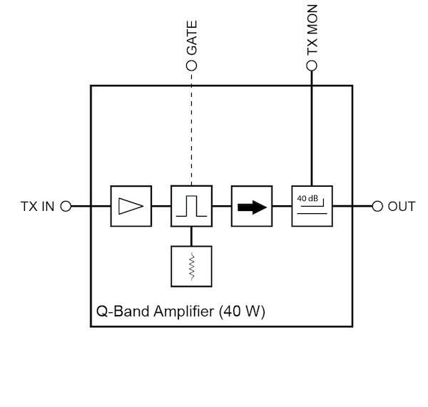
The Bridge12 AMP-Q40 is a 40 W solid-state microwave amplifier for Q-Band (35 GHz) pulsed EPR spectroscopy. The amplifier can fully replace a TWT amplifier and in combination with the Bridge12 QLP-1.6 probe is a great combination for pulsed dipolar EPR spectroscopy.
Note
The expected pulse length for a 180º-pulse, using a maximally overcoupled Bridge12 QLP-1.6 resonator is 16 ns.
A schematic of the amplifier is shown in the figure above. The amplifier has an integrated gate, isolator, and coupler. The input connector for the amplifier is a 2.92 mm connector, while the output is a WR-28 waveguide output.
Back Panel Connections
The Bridge12 AMP-Q40 can fully replace a TWT amplifier. The following connection to the spectrometer need to be made:
Microwave Input (TX IN): Input connection of the amplifier. This needs to be connected to the output of the EPR bridge. 2.92 mm connector.
Microwave Output (OUT): Output connection of the amplifier. This either needs to be connected to the circulator extension (Bridge12 Q-Band spectrometer) or to the input of the EPR bridge. If you are unsure please contact Bridge12 at support@bridge12.com. If your EPR bridge requires a 2.92 mm input connection, we recommend installing a waveguide to coax adapter.
Gate: Amplifier blanking. This gate is active HIGH and needs a trigger pulse from the EPR bridge.
Microwave Monitor (TX MON): Monitor output of the amplifier. This is the same signal that is sent to the probe but attenuated by 40 dB. The signal can be used to monitor the microwave pulses or to characterize the amplifier performance.
15 Pin D-Sub Connector: Control and monitor signals of the amplifier. For a detailed pin out see tabel below.
Operating Instructions
Warning
Do not obstruct the airflow of the cooling air. This can lead to overheating of the amplifier and possible permanent damages.
Power Up Procedure
Make sure that no microwave pulses are sent out by the EPR bridge.
Turn on the amplifier.
Wait a few minutes for the amplifier to warm up. For optimum, stable performance we recommend to leave the amplifier for about 20 minutes for the internal temperature to stabilize. The amplifier has an internal delay of 5 s. You need to wait at least for this time before sending the first microwave pulses.
Apply gate and microwave pulses.
Power Down Procedure
Make sure that no microwave pulses are sent out by the EPR bridge.
Turn off the amplifier.
Pulse Timing
Warning
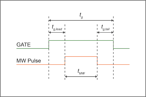
Do not Hot Switch the amplifier. Hot Switching occurs, when the blanking gate is disabled while sending a microwave pulse. This can lead to permanent damage of the internal protection circuit of the amplifier. Please see the timing diagram below.
Please refer to the timing diagram and the values below for recommended pulse timing.
Gate lead, tg,lead > 100 ns (200 ns recommended)
Gate tail, tg,tail > 20 ns (50 ns recommended)
Maximum duty cycle: 20%
Maximum pulse length: 10 µs
ATTENTION: DO NOT HOT SWITCH AMPLIFIER
15 Pin D-Sub Back Panel Connector
Pin Number
Name
Function
Initial State
Description
1
Reset
Control
-
Resets PA when logic LOW is applied and released
2
Gate Disable
Control
LOW
Applying a HIGH signal disables gate of amplifier
3
Drain Disable
Control
LOW
Applying a HIGH signal disables drain of amplifier
4
RF IN Over
Indicator
LOW
Pin will be latched to HIGH when input signal is to high
5
Temp Over
Indicator
LOW
Pin will be latched to HIGH when maximum amplifier temperature is exceeded
6
Current Over
Indicator
LOW
Pin will be latched to HIGH when drain current limit is reached
7
ID Imbalance
Indicator
LOW
Pin will be latched to HIGH when an imbalance in the drain current of the combining branches occurs
8
PA Off Alarm
Indicator
LOW
Pin will be latched to HIGH when any of the protection limits are reached
9
-
not connected
-
10
-
not connected
-
11
-
not connected
-
12
-
not connected
-
13
-
not connected
-
14
+5 V
Power Supply
+5 V
+5 V DC power supply for reference. Mac. 400 mA available
15
GND
Ground
GND
Electrical ground
1.4 - Magnets
Superconducting- and Electromagnets for EPR Spectroscopy
1.4.1 - Superconducting Magnets
Superconducting Magnets for EPR Spectroscopy
Many Bridge12 (high-field) EPR spectrometers use superconducting magnets manufactured by CRYOGENIC LTD. The magnet system comes with extensive documentation.
All information provided here is specific to superconducting magnets specifically manufactured to be used in Bridge12 instruments. In addition, most instructions here describe procedures for day-to-day operations.
1.4.1.1 - Magnet Installation
Supporting Information for Magnet Installation
During the initial installation of the spectrometer, the magnet will be installed by an engineer from Cryogenic Ltd. Once the magnet is installed and passes the customer acceptance test no further installation steps are necessary.
If you have any more questions please reach out to:
Please make sure to read the instructions for cooling down the magnet carefully. Make sure you don’t have any questions and all required equipment is in place.
These instructions are not to be used for initial cooling down of the magnet. For these instructions it is assumed that the magnet was properly decommissioned by Bridge12 or CRYOGENIC.
If you have additional questions please do not hesitate to reach out to Bridge12 or CRYOGENIC.
Required Equipment
For cooling down the magnet or recharging the helium reservoir of the integrated VTI (iVTI) the following additional equipment is required:
Vacuum pump, preferable a turbomolecular pump with a capacity of 12 m3/hr.
Various vacuum hoses, matching center rings and clamps
High grade helium gas (grade 5). This is only required for recharging the helium compressor or the helium reservoir of the iVTI. For changing the sample regular grade helium gas is sufficient.
Hoses, fittings, pressure regulator, etc. to connect the helium cylinder to the iVTI.
1. Evacuation of the Magnet Cryostat
The magnet cryostat has a single vacuum space which is evacuated via the bellows sealed valve fitted to the cryostat top plate. As a guide, this space should be evacuated using a pump with a capacity of at least 12 m3/hr and a base pressure of <10-4 mbar. Outgassing of the superinsulation occurs whenever the cryostat is allowed to warm up to room temperature. Also, after a magnet quench it is sometimes necessary to evacuate the magnet cryostat, especially if you can’t reach the normal base temperature of the magnet after a quench.
To evacuate the magnet cryostat, connect a vacuum pump to the vale located at the top of the cryostat. Start the vacuum pump and once the pump has reached its base pressure open the valve to the magnet cryostat. The cryostat should be pumped down to a pressure of <10-3 mbar before attempting to cool down. If the pressure decrease is slow, this may be an indication of moisture in the superinsulation which will require more extended pumping of the interspace.
Under normal circumstances there is no need to vent the vacuum space to atmospheric pressure. It is strongly recommended to not vent the vacuum space to decrease the time it takes for the magnet to come up to room temperature. If you have to vent the magnet cryostat please consult the instructions in the magnet manual or contact CRYOGENIC.
2. Prior Checks Before Cooling Down the Magnet
Before cooling down the magnet, please observe the following operational checks:
Magnet
The cryostat vacuum space is adequately evacuated to a base pressure of <10e-3 mbar
The compressor is connected to the electrical mains according to the supply information on the compressor housing. Please refer to the compressor manual for further information regarding power requirements.
Adequate water cooling is provided for the compressor (water-cooled versions only). Please refer to the compressor manual for the correct specification for the water circuit.
Both ends of the flexible hoses connecting the compressor to the cold head are properly tightened. Make sure the charcoal trap is installed. Please use the supplied tools to tighten all connections.
The electrical lead from the compressor to the cold head is connected.
The current leads running from the magnet power supply are securely attached to the magnet terminals.
The magnet coil is electrically isolated from the cryostat. To check this, measure the resistance between a magnet current terminal and one of the cryostat top plate outer fixing bolts. A value of ≥ 500 kΩ is typical.
The temperature monitors/controllers are installed properly and the lead(s) are connected.
The static helium pressure in the compressor is correct to ensure it is at the recommended value. Please refer to the compressor manual for the correct specification of the helium pressure. If the pressure is lower than expected please follow the instructions in the compressor manual before starting the compressor.
The system is properly positioned such that there are no significant ferromagnetic objects (e.g.; steel beams, pumping stations etc) close to the cryostat. It should be noted that structural supports on the floor must also be considered when positioning the cryostat. Please contact CRYOGENIC if you are unsure about the possible influence of magnetic objects adjacent to the system.
integrated VTI (iVTI)
The dry pump for the iVTI is connected to an outlet. At this time, the dry pump is not powered on.
The external gas reservoir must be charged to the correct pressure with clean helium gas and connected to the cryostat (see system specification). The reservoir is connected to the iVTI gas circuit via a face-sealing connector.
It is recommended that the flow through the iVTI is checked at room temperature prior to cooling down the magnet.
Make sure the dry pump bypass valve (V16) is closed and th helium reservoir valve (V12) is opened.
Make sure the iVTI butterfly valve is open
Switch on the dry pump and pumping for a short time on the iVTI head with the needle valve fully open and circulating gas through the external dump as in normal operation at cold temperatures. The expected flow should be in the range of 5-15 mbar.
Having checked the room temperature flow, switch oof the dry pump
Open the bypass valve (V16). This allows gas to circulate via natural convection throughout the gas circuit during the cooldown of the magnet. The convective flow helps to cool the internal components of the gas circuit whilst minimizing the wear of the pump.
Charge the static column, the space where the resonator is located, to 1 atmosphere of clean helium gas from an external source of helium. The gas is necessary to conduct heat from the wall of the static column and maintain a small temperature differential between the helium flowing in the annular space around static column and the sample probe. It is recommended to charge the static column prior to cooldown as once the system is cold it is more difficult to judge the quantity of helium being added due to condensation of the gas as it enters the column. The approximate volume of the static column is .05 litres.
Cooling Down the Magnet
Once all prior checks have been completed (see instructions above) the magnet cooldown can be started. It is recommended, that the system monitor is started to log all temperatures during the cooldown process.
Cooling the magnet is simply a matter of starting the helium compressor:
Turn the switch located on the back of the compressor into the ON position.
Press the ON button to start the compressor.
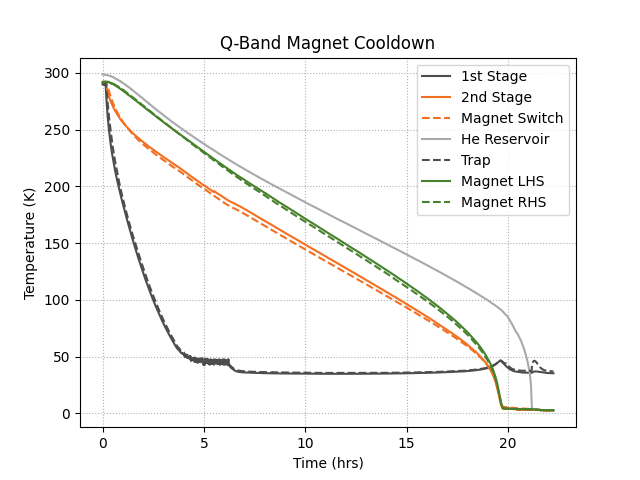
Typically the 1st stage of the cryocooler will cool fastest followed by the 2nd stage and then the magnet. For this magnet, the cooldown time is typically about 22 hrs. It should be noted that initially, the operating pressure at the compressor will be high and then reduce (typically by 20 %) as the magnet temperature drops and the cryocooler is required to do less work to remove heat from the system. Once the base temperature of the magnet is achieved the magnet may be energized.
Temperatures of a Typical Magnet Cooldown
Temperatures for a typical cooldown of the magnet are shown in the figure above. The following table has shows some typical temperatures once the magnet is at its base temperature.
Q-Band Magnet with iVTI Base Temperatures
Parameter
Value
Parameter
Value
Cryocooler 1st stage
36.2 K
Persistence Switch
3.0
Cryocooler 2nd stage
3.0 K
Helium pot (Not heated)
3.0 K
Magnet LHS winding
3.0 K
Helium pot (heated)
3.2 K
Magnet RHS winding
3.0 K
Charcoal trap (not circulating)
46.6 K
Checking the iVTI Operation
Once the magnet has avhieved base temperature:
Close the bypass valve (V16) across the dry pump.
Make sure the cryostat heater is switched off.
Start the dry pump.
Adjust the needle valve to a pressure of approximately 6 mbar at the iVTI pump port. Please note the needle valve may require several further adjustments as the temperature profile within the flow circuit varies whilst steady-state flow conditions are established in the circuit.
For further information/instructions on how to operate the iVTI please see the section about operating the iVTI.
1.4.1.3 - Warming Up the Magnet
How to warm up the magnet
Warning
Please make sure to read the instructions for warming up the magnet carefully. Make sure you don’t have any questions and all required equipment is in place.
If you have additional questions please do not hesitate to reach out to Bridge12 or CRYOGENIC.
Once experiments are finished and the user anticipates some considerable downtown when no experiments are planned the magnet can be warmed up to room temperature. To warm up the magnet:
Make sure the field is at 0 T. This can be verified either in the spectrometer control software or on the front panel of the magnet power supply.
Make sure the spectrometer logger is running and is recording vital data of the system.
To switch off the helium compressor press the off switch located on the back of the device. Once the compressor is switched off, the magnet starts immediately to warm up. It is recommended that the system then be left to attain room temperature naturally which will take approximately 36 - 48 hours.
Warning
Do not disconnect the compressor hoses for any reason during the warm-up of the system. The gas in the cryocooler head must be allowed to expand into the reservoir volume located in the compressor.
It is common practice to break the interspace vacuum when required to warm a cryostat more rapidly than would otherwise occur naturally. CRYOGENIC strongly discourages users from venting the vacuum interspace for any reason.
The radiation shield may collapse if subject to an appreciable pressure differential (i.e. by opening the cryostat vacuum valve too quickly).
When the user is ready to continue experiments the magnet needs to be cooled down. Please follow the instructions in the Magnet Cooldown Section.
1.5 - Integrated VTI (iVTI)
1.5.1 - Overview of the iVTI Operation
How the Integrated VTI (iVTI) Works
iVTI - How it Works
The integrated Variable Temperature Insert (iVTI) is a liquid cryogen-free (dry) cryostat built into the superconducting magnet of the EPR spectrometer. It operates by circulating helium gas around a closed-loop circuit cooled by the same cryocooler that is used to cool the superconducting magnet coil. The iVTI can operate continuously and in conjunction with the magnet.
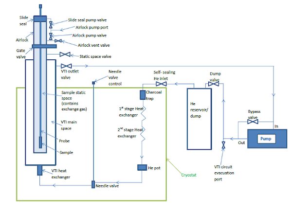
Schematic of the iVTI
A schematic of the iVTI is shown above. High quality helium gas (grade 5) is stored at room temperature in the helium reservoir and a dry (oil-free) pump drives drives the circulation of the helium gas through a closed cycle circuit. Under normal operations, the bypass valve (V16) is closed and the helium reservoir valve (V12) and iVTI outlet valve (V11) is open. The helium gas passes from the helium reservoir and into the iVTI circuit via the self-sealing helium gas inlet.
Once the helium gas enters the magnet space, it first passes through a charcoal filter to remove any impurities within the gas. It then flows through the first stage heat exchanger which cools the gas to ~40K. The gas then passes to the second stage heat exchanger
where it is cooled further to below 4.2K and condenses in the helium pot. The helium pot has an integrated heater to keep the pot at a recommended temperature of 3.1 K.
To cool the cryostat space, the liquid helium then flows across the needle valve, at which point it expands and cools further to approximately 1.6K. The cooled gas/liquid mixture then passes through the iVTI heat exchanger where the helium is heated to the required temperature. The helium gas flows upwards in an annular space surrounding the static column (containing the EPR probe) to the top of the iVTI where it exits and is circulated through the pump and exhausts back to the dump vessel.
The probe is cooled using an exchange gas, which is cooled at the wall of the static column.
The temperature inside the cryostat is regulated using the iVTI heater located at the bottom of the static column, and the heating power is regulated by the temperature controller. To achieve the most accurate temperature at the position of the sample, all Bridge12 EPR probes are equipped with a calibrated Cernox temperature sensor. This sensor is located as close to the sample as possible for accurate temperature readings and this temperature is used to control the heater power in a feedback loop.
If the probe is removed from the cryostat, the temperature can be regulated using the internal iVTI temperature sensor. Note, that the iVTI temperature is not necessarily equal to the sample temperature.
Integrated Heaters
The magnet system with integrated VTI has in total three internal heaters that are all connected to the temperature controller (typically a LakeShore Model 350). The following table summarizes the function of the heater and gives some default operation parameters.
Heater
Description
Heater 1 (VTI)
The VTI heater is used to regulate the cryostat temperature. Typically, the heater control loop is connected to one of the temperature sensors (this is done in the settings for the temperature controller). For the Q-Band spectrometer the user has the option to control the cryostat temperature using the temperature sensor of the VTI or the one integrated into the EPR probe. Bridge12 recommends using the temperature sensor of the EPR probe for accurate temperature readings.
Heater 2
Not used
Heater 3 (Helium Pot)
During operation some the helium of the VTI used for cooling is condensed inside the helium pot and the flow of helium is controlled by the needle valve (see figure above). Under normal conditions, the temperature of the helium pot should be kept at around 3.3 K. To achieve this temperature the heater output power should be set to a value of about 5 to 10 % (open loop) to maintain that temperature. This value only needs to be changed if the user wants to go to very low temperatures (e.g. < 5 K) and the user should first read the instructions in the manual to set the temperature of the helium pot.
Heater 4 (Charcoal Trap)
During normal VTI operations the helium passes through an activated charcoal filter to remove any residues (oxygen, nitrogen, etc.) from the helium gas used for cooling. After a while this charcoal filter needs to be degassed (cleaned) using the charcoal heater. This is a low power heater and the heater can be ramped up to 100%. While ramping up the heater, please monitor the temperature of the charcoal trap in the logging system. During normal operations, the charcoal heater is off.
1.5.2 - Getting Started with the iVTI
Getting Started with the iVTI
Important
Before operating the iVTI please familiarize yourself with the principle of operations described in the section iVTI Overview.
The following section provides information about day-to-day operation of the cryostat. If you need assistance troubleshooting iVTI operations, please first consult the manual or contact Bridge12 or CRYOGENIC.
Prior Checks Before Operating the iVTI
Warning
Do not use excessive force or overtighten the needle valve as this can lead to permanent damages of the valve.
Note
If the needle valve is closed and open again, a faint clicking sound is heard as the needle pulls away from the needle valve seat.
Once the magnet has achieved its base temperature the following checks should be performed prior to operating the iVTI:
Make sure the dry pump bypass valve (V16) is closed.
Make sure the helium reservoir valve (V12) and the iVTI outlet valve (V11) are open.
Start the dry pump and adjust the needle valve to a pressure of approximately 5-8 mbar at the head of the iVTI. Please note the needle valve may require several further adjustments as the temperature profile within the flow circuit varies whilst steady-state flow conditions are established in the circuit.
Within a short period of time, the cryostat should reach its base temperature of ~ 1.8 K.
Setting an optimum flow rate requires some experience from the user. The factors that must be considered are:
If the flow rate is too low the 2 K base temperature of the iVTI may not be achievable, as the available cooling power of the gas may be too low.
If the flow rate is too high the cryocooler second stage temperature will rise which may affect the maximum ramp rate of the magnet.
If the flow rate is too high the cryocooler may not condense at a fast enough rate. This leads to rapid boiling of the condensed gas in the circuit and a rapid pressure rise of the circuit.
Typically the iVTI can operate with a single needle valve setting over its whole temperature range. However, if a rapid cooldown is required the user can increase the flow and then subsequently re-adjust the needle valve to give a lower flow setting once the iVTI has cooled close to the required temperature.
1.5.3 - Operating the iVTI
How to Operate the iVTI
Important
Before operating the iVTI please familiarize yourself with the principle of operations described in the section iVTI Overview.
The following section provides information about day-to-day operation of the cryostat. If you need assistance troubleshooting iVTI operations, please first consult the manual or contact Bridge12 or CRYOGENIC.
Schematic of the iVTI
The iVTI operates by circulating helium gas in a closed-loop circuit. A schematic of the circuit is shown above. The following instructions assume the magnet is at its base temperature and the iVTI has passed operational checks.
Cooldown of the iVTI
To cooldown the cryostat follow these instructions:
Make sure the dry pump bypass valve (V16) is closed.
Make sure the helium reservoir valve (V12) and the iVTI outlet valve (V11) are open.
Start the dry pump and adjust the needle valve to a pressure of approximately 5-8 mbar at the head of the iVTI. Please note the needle valve may require several further adjustments as the temperature profile within the flow circuit varies whilst steady-state flow conditions are established in the circuit.
While the cryostat cools down, the pressure of the helium reservoir will decrease as more helium condenses in the helium pot.
Setting the Cryostat Temperature and Regulating the Helium Flow
Setting the Temperature
The temperature at the position of the sample is set at the temperature controller. This can be done either manually at the front panel of the temperature controller or through the spectrometer control software SpecMan4EPR. Under normal operations, when there is an EPR probe installed, the temperature of the cryostat is regulated based on the probe temperature sensor readings to give the most accurate control over the temperature at the position of the sample. Once the temperature is set, either on the front panel or through SpecMan4EPR, the user needs to adjust the helium flow by adjusting the needle valve. However, once the desired temperature is reached, no further optimization is required.
Optimization of the temperature controller PID and heater range parameters is beneficial if the ultimate system performance is to be achieved. The parameters may vary depending upon the flow rate established in the circuit. Typical starting values for the PID settings are 250,120,30 which will provide reasonable control over the whole temperature range. However, the user is encouraged to adjust PID settings to further optimize the system as an experience of the iVTI is established. The heat exchanger is fitted with a heater (30 Ohm / 30 W). Under no circumstances should a current greater than 1A be applied to the heat exchanger heater, as it will fuse the leads.
Setting the Needle Valve for Optimum Flow Control
The needle valve creates a controllable impedance for the helium circulation. It is set initially and thereafter should need only occasional adjustment. A dial gauge is fitted at the top of the iVTI to allow the user to set and monitor the flow rate (directly related to pressure). A pressure between 5 and 15 mbar at the top of the iVTI is recommended. The optimum value is specific to each system.
Under normal conditions, a pressure of about 10 mbar can cover a wide range of temperatures. Especially, for experiments that are performed at about 50 to 60 K, the position of the needle valve rarely has to be changed.
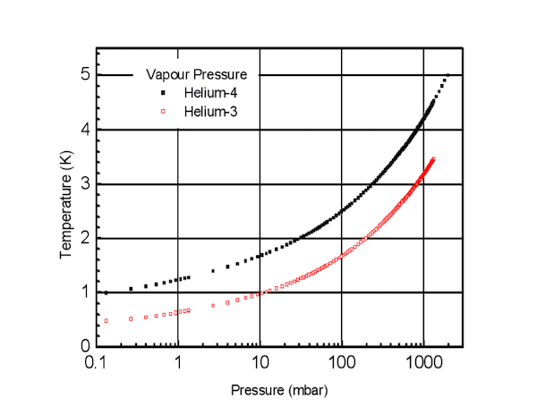
To operate at temperatures below 10 K, the pressure may have to be adjusted using the needle valve. In this case, the optimum value will correspond to the vapour pressure curve as shown in the figure below.
Helium Vapor Pressure
In general, if the helium flow rate is too low there may not be enough cooling power available from the circulating helium and the system may not reach the base temperature of the iVTI. A slightly too high a flow rate and the system will not reach base temperature because it is not following the vapour pressure curve.
However, if the flow rate is far too high the amount of heat that needs to be extracted from the circulating helium will exceed the cooling power of the cryocooler. In this case, the temperature of the cryocooler 2nd stage, magnet and helium pot will increase and the liquefaction of helium in the iVTI circuit will slow or stop. Under these circumstances, the helium pot will eventually empty preventing the iVTI from achieving base temperature. The associated increase in temperature will also affect the magnet ramp rates.
It should be noted that the helium flow is also affected by the impedance of the tubes close to the iVTI heat exchanger. The overall impedance depends on the temperature of the heat exchanger. A higher driving pressure is needed between the helium pot and the iVTI when the iVTI is at a high temperature than when it is at a low temperature. The liquid helium in the helium pot is effectively in equilibrium. So the pressure of the gas above the liquid in the helium pot follows the vapour pressure curve for helium 4 shown in the figure above. Since the inlet circuit has a low impedance, the pressure in the helium reservoir is close to that at the helium pot and can be used as a gauge as to how much helium has been condensed into the pot. A heater on the helium pot is used to control the temperature of the helium pot and hence control the driving pressure. The temperature is set to a recommended value of 3.1 K. The helium pot temperature is controlled via a software PID loop.
Changing the Sample
During the process of changing the sample, the iVTI circuit will continue to run and the dry pump should not be switched off. To change the sample, follow these instructions:
Removing the Sample
If you want to insert/replace a new sample, make sure the sample is properly mounted on the sample stick. If you want to remove the sample without inserting a new sample, make sure you have a blind plug handy.
Make sure the experiment is finished.
Make sure helium purge gas is available and the pressure regulator is set to the correct value. For the sample exchange circuit, the pressure regulator should be set to a pressure of 3-5 psi.
Open the valve to the cryostat, located at the top of the magnet and observe the pressure inside the cryostat. You should charge the cryostat space to about 1 psi. A safety valve, located close to the valve will release all excess pressure.
Loosen the nut securing the sample stick.
Slowly pull out the sample stick. The sample stick has holes at the top and bottom of the G10 section (green). Once the top hole passes the nut securing the sample stick, cold helium gas will exit the hole. Pull the sample stick out of the probe and properly store the sample. While the purge gas is running, air is prevented to enter the sample space.
Inserting the Sample
With the purge gas running, insert the sample stick into the probe.
Slowly lower the sample stick into the probe. Once the bottom venting holes of the sample stick have past the nut securing the sample stick the helium purge gas will exit at the top holes of the sample stick. Wait for a couple seconds to purge the space inside the of the sample stick.
Optionally, open the nut at the top of the sample stick to purge the space inside the stainless steel section of the sample stick.
Slowly push the sample stick into the resonator. At this point, the user should also monitor the resonator tuning in the control software. Once the sample tube is entering the resonator, the frequency will shift to a lower value. Push the sample stick until it is properly seated at the top of the resonator.
Tighten the nut securing the sample stick. Important, this only needs to be hand-tightened. Do not use any tools to tighten this nut.
Close the valve to the helium purge gas supply.
Switch on the diaphragm pump to evacuate the sample space. Lower the pressure to about 200 - 500 mbar. The exact value depends on desired temperature and will require some user experience.
Close the valve to the iVTI located at the top of the magnet.
Turn off the diaphragm pump.
Once the sample is loaded into the resonator make sure to close all valves to the helium supply for purging.
1.5.4 - Troubleshooting iVTI Operation
How to Operate the iVTI
Important
Before operating the iVTI please familiarize yourself with the principle of operations described in the section iVTI Overview.
The following section provides information about day-to-day operation of the cryostat. If you need assistance troubleshooting iVTI operations, please first consult the manual or contact Bridge12 or CRYOGENIC.
Blockage in the iVTI Circuit
The most likely cause of abnormal iVTI performance is a blockage in the iVTI circuit due to ingress of air.
Symptoms of a iVTI partial blockage before the helium pot can include:
Reduced flow at a given needle valve setting.
Reduced pressure at the iVTI pumping side for a given needle valve aperture.
Increased pressure at the external helium reservoir.
Decreased temperature of the 2nd stage and helium pot.
The pressure in the helium reservoir increases as the partial blockage limits the flow of helium through the inlet heat exchangers. The 2nd stage and helium pot temperatures may fall as the cryocooler heat load is reduced due to the lower helium flow rate at the 2nd stage.
Symptoms of a blockage after the helium pot are similar; however, in this case, the helium reservoir pressure may fall as the helium charge is condensed into the system with a reduced flow returning to the reservoir.
If a blockage is suspected the following actions are recommended:
Heat the iVTI to room temperature. In some cases, this may clear the blockage.
If the blockage persists, please follow these steps:
Once the iVTI is at room temperature, disconnect the helium reservoir hose at the face-sealing connector on the cryostat.
Connect an external pump to the face-sealing connector of the cryostat using the fitting that was provided with the system. This connection provides the most efficient pumping of the inlet circuit which is the most likely location for any blockage to occur.
Close the valve at the head of the iVTI (V11) to the dry pump and open the needle valve fully.
Pump the iVTI via the external pump and switch off the compressor.
Heat the charcoal trap using the temperature controller and maintain it at 300 K.
Wait for the 2nd stage to rise in temperature above 90 K.
Turn off the charcoal heater, isolate the external pump and restart normal flow through the iVTI circuit.
If the blockage persists, continue to warm the system to room temperature and replace the helium of the iVTI circuit as outlined below.
Replacing the Helium in the iVTI Circuit
If contamination or loss of helium in the iVTI circuit is suspected please follow these instructions to replace the helium charge:
Make sure the system is at room temperature and the dry pump is not running.
Connect a T-connector to the plug valve on the exhaust side of the dry pump. One arm of the T should be connected to a clean helium source with an in-line valve, and the other to a pump via a valve. The helium source should be either a bottle of high purity gas (99.95%, grade 5) or the boil-off gas from a helium storage vessel. Do not use standard (balloon) grade bottled helium for this purpose as this can have a high moisture content.
Open the connection to the external pump and pump out the helium reservoir. Once the pressure is low enough (< 1e-3 mbar>) activate the dry pump and use it to purge the internal iVTI circuit.
Close the valve to the external pump and fill the reservoir to a pressure of +1psi above atmospheric pressure with pure helium gas.
The system is now ready for cooldown and operation.
1.6 - The Bridge12 Q-Band Spectrometer
Online documentation for the Bridge12 Q-Band pulsed EPR spectrometer.
1.6.1 - Overview
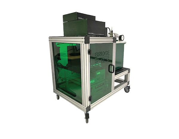
Compact Q-Band EPR Spectrometer
The Bridge12 Q-Band spectrometer is a compact EPR spectrometer for pulsed EPR spectroscopy.
The main features of the system are:
Compact magnet with integrated liquid cryogen-free (dry) cryostat (more information)
Modern microwave electronics. Pulse sequences are entirely controlled by an AWG (more information)
Getting started with the Q-Band spectrometer SpecMan4EPR
In this section we give a general overview how to operate the Bridge12 Q-Band pulsed EPR spectrometer, which will include the following steps:
Loading the sample into the spectrometer
Optimizing the microwave pulse parameters
Record an echo-detected field sweep EPR experiment
Perform a PELDOR/DEER experiment
All experiments were performed on our in-house spectrometer, using a sample of a ruler molecule with a concentration of 100 µM in polystyrene. Experiments were performed at a temperature of 50 K.
Important
These are sample instructions recorded on equipment in our lab. Actual parameters may vary depending on your specific system configuration, sample, or sample temperature.
This documentation was prepared using SpecMan4EPR version 3.6.4. If you use a different version some features are maybe named differently or the layout of some windows has changed.
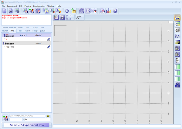
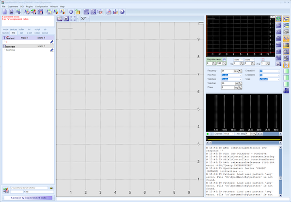
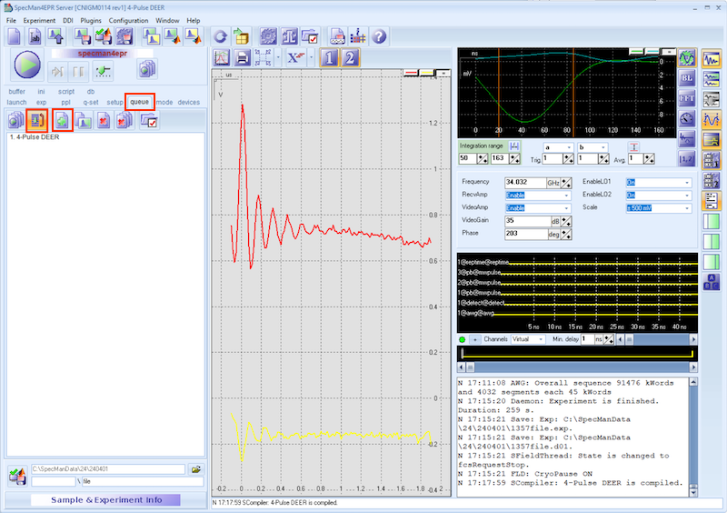
Preparing SpecMan4EPR
When you first start SpecMan4EPR, the software will make sure it can connect to all devices. Once the initialization routine finishes you will see a window very similar to the one shown in the figure below.
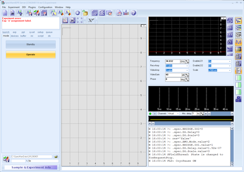
We recommend to open the following windows to operate the spectrometer:
Open the Scope Window and activate the digitizer trace. This will be helpful to see the integration limits for the digitizier.
Open the Pulse Programmer window to show the pulse sequence.
Open the top User Panel, this will give you convenient access to bridge parameters such as the microwave frequency, video amplifier gain, or the microwave phase.
Optionally, open the Log Window. This is helpful to see messages from the SpecMan4EPR software.
Once you opened all these additional panels, the SpecMan4EPR window should look similar to the one shown below.
1.6.2.1 - Inserting a Sample and Adjust the Resonator Coupling
How to insert the sample into the spectrometer
The following section provides a step-by-step procedure how to insert the sample into the EPR probe and adjust the iris coupling of the resonator.
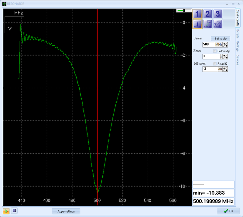
To confirm that the sample is inserted into the microwave resonator correctly, we will observe the microwave tune dip of the resonator.
Inserting the Sample
Make sure SpecMan4EPR is running.
To insert the sample follow these steps:
Switch the spectrometer into operate mode
From the Experiment Panel select the mode tab
Click the Operate button. This will enable all synthesizers
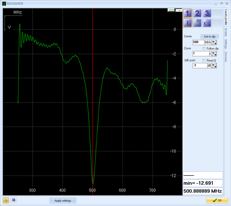
Open the resonator tune window (RESONATOR plugin) from the plugins window
Start the tune sweep by clicking the run button (green arrow on bottom left)
Make sure the resonator is critically coupled. For this, the resonator iris is completely inserted into the resonator. This corresponds to a micrometer reading of 0 mm.
To insert the sample:
Make sure the helium gas pressure inside the cryostat is slightly above atmospheric pressure (> 0.1 bar). Note, the pressure gauge shows a value of 0 bar, when the pressure inside the cryostat is close to atmospheric pressure.
Once the pressure in the cryostat is slightly above atmospheric pressure, it is safe to remove the bling plug. For this loosen the nut and pull out the plug. You will feel a stream of cold helium gas exciting the cryostat. This will prevent air and moisture entering the sample space.
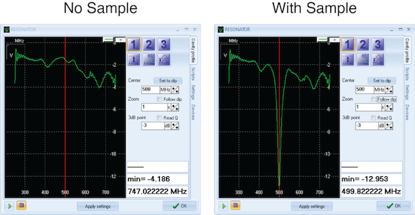
Slowly insert the the sample stick and lower it into the resonator. The sample stick has holes at the top and the bottom to release the helium gas coming from the probe. While lowering the sample stick, observe the tuning picture of the resonator. Once the sample enters the resonator, the tuning dip of the resonator will be visible (see figure below).
Once the sample is fully inserted into the resonator, tighten the nut at the top of the probe that holds the sample stick. This nut should just be hand-tight. Do not use any tools (e.g. pliers) to close the nut.
Close the valve to the helium gas supply.
Start the pump and open the valve to the pump to lower the pressure inside the cryostat to about -0.5 bar. The exact pressure is not important.
Close the valve to the pump and wait for a couple minutes until the temperature inside the cryostat stabilizes.
In side the tune window you can zoom into the tune picture by clicking the up and down buttons.
Overcoupling the Resonator
For pulsed EPR experiments the resonator must be overcoupled to reach the maximum resonator bandwidth.
Before you adjust the resonator iris to overcouple the resonator, make sure the microwave frequency (red vertical line) is set to the tuning dip. The microwave frequency is adjusted in the Control Panel (see figure above).
Slowly turn the micrometer screw to overcouple the resonator. This will raise the iris and the tuning dip will get broader. The tune dip will also shift ub by about 90 MHz. For maximum overcoupling set the height of the iris to 7 mm.
For DEER experiments on nitroxide-based spin labels you don’t have to adjust the microwave frequency. The shift of the dip is about 90 MHz, which corresponds to the frequency separation of the pump and observe pulse. When using different paramagnetic species the frequency may have to be adjusted. However, keep in mind, the resonator bandwidth is > 400 MHz for the Bridge12 QLP probe.
To exit the tune mode, click the stop button (click the square icon, bottom left) and click the OK button to close the window.
The spectrometer is ready for the first experiment.
1.6.2.2 - Optimizing the Microwave Pulse Parameters
How to optimize the microwave pulse parameters for PELDOR/DEER experiments
In this section we provide the general procedure how to optimize the microwave pulse parameters for the PELDOR/DEER experiment.
Set the Magnetic Field
Use the microwave frequency that was set in the microwave bridge Control Panel to calculate the maximum field for a nitroxide radical. This can be done using the provided Python script.
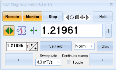
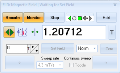
In this example the microwave frequency is 34.032 GHz and the script returns a field value of 1.21896 T.
Next, open the window to control the field. From the DDI menu select Set Field form, FLD.
Enter the field value and click the Set Field button.
Wait until the desired field value is reached. When the magnetic field is sweeping, the temperature of the Magnet Switch will typically rise from about 5.9 K to about 8 K. Once the desired field is reached, the temperature returns to its base temperature of about 5.9 K.
Close the magnet control window.
Optimizing the Pulse Parameters
To optimize the pulse parameters follow these steps:
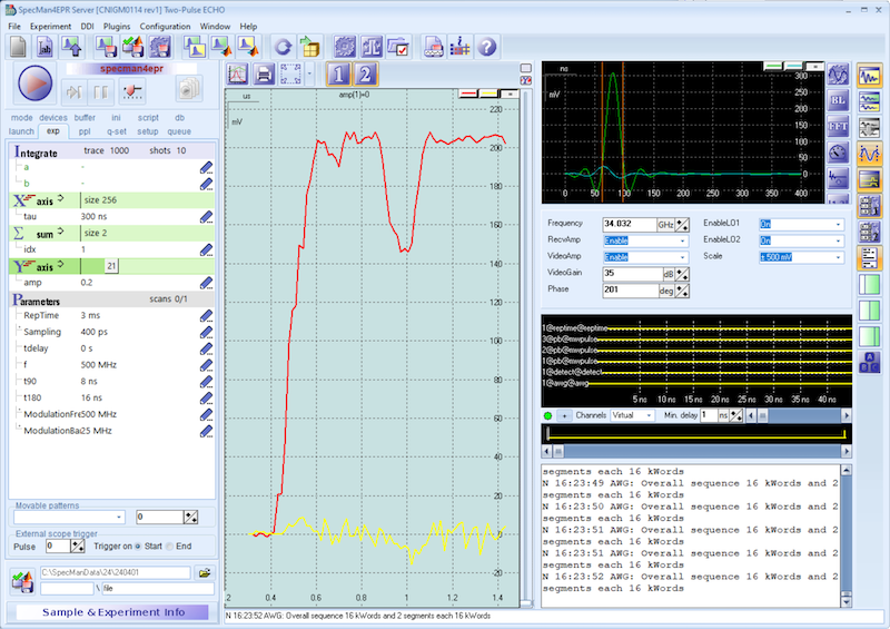
Load a new experiment. From the File menu, select New Experiment. Scroll to the Two-Pulse Echo experiment and click on it to load the experiment. This will load some default pulse parameters, which will be a good start for the optimization.
Next, start the pulse sequence by hitting the Tune button. Once the experiment starts, you should see an echo in the Scope window to the left.
In the next step we will adjust the video amplifier gain and the microwave phase. This is an iterative process and you have to adjust both parameters. Make sure the Modulation Frequency parameter is set to 500 MHz.
In the microwave bridge Control Panel adjust the video amplifier gain. Observe the echo amplitude and set the video amplifier gain to a value so the echo amplitude is not clipped.
In the same window adjust the microwave phase to maximize the echo amplitude (real part of the complex signal, green trace).
The video amplifier gain should be adjusted to a value that the echo amplitude is about 75 % of the maximum (horizontal red line). For small echo amplitudes, you can also adjust the scale in the same window. This will adjust the input scale of the digitizer.
In the next step, we will find the optimum value for the microwave power. SpecMan4EPR allows the user to make almost every variable of the experiment an axis of the experiment. We will use this feature of the software to find the correct pulse amplitude.
Right click on the amp variable in the Parameter section and select Y axis to assign the parameter to the y axis.
In the section for the y axis, set the size of the axis to 101 points.
In the line below, set the sweep range to "0 step 0.01". This will you to step the amp parameter from 0 to 1 in steps of 0.01 using the slider.
To start the experiment, click the tune button.
Move the slider with the mouse to maximize the echo amplitude.
Find the optimum pulse amplitude for a two-pulse echo using 8 and 16 ns for the pi/2 and pi pulse, respectively. In this example the optimum value is at 0.2 (21st step).
Change the pulse length the for 90º and 180º pulse to 16 and 32 ns, respectively, and repeat the optimization. In this example the optimum value for the 16/32 echo is at 0.08. This value should be approximately half of the value determined for the 8/16 ns echo.
While the tune mode is running, SpecMan4EPR will integrate the area of the echo and record the value in the display. Observe the value (red trace in figure below) and optimize for the maximum echo amplitude.
Once you found the optimum values stop the tune mode by clicking the tune button.
Record reference T2 decay
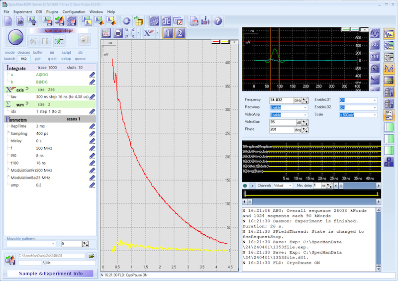
In the next step, we will record a two-pulse echo decay as a reference spectrum. This will give you and idea of the setting for the maximum dipolar evolution time. To record the T2 decay follow these steps:
Reload the experiment. From the File menu, select New Experiment. Scroll to the Two-Pulse Echo experiment and click on it to load the experiment.
Set the amp parameter (pulse amplitude) to the value determined above. In this example we use the parameters for the 8/16 ns echo.
Hit the run button to start the experiment.
It will take about 15 s to compile the pulse sequency and upload it to the AWG. Once the sequence is uploaded the experiment will start and the results are shown once the experiment finishes (see figure below). Overall duration for this experiment is about 26 s.
For this particular sample we pick a maximum dipolar evolution time of about 2 µs.
How to record an echo-detected field sweep spectrum
In this section we will provide general instructions on how to record an echo-detected field sweep spectrum.
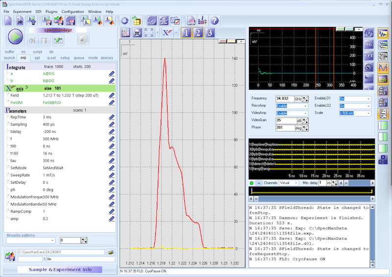
First, load a new experiment. From the File menu, select New Experiment. Scroll to the Field Sweep Echo in Set Mode experiment and click on it to load the experiment.
When you load the experiment SpecMan4EPR will set all experimental parameters to the default values loaded from the template. Adjust the parameters to the values determined in the previous experiments, such as pulse length, pulse amplitude, …
Under X-axis set the field range and number of points for the experiment. To get started use the field sweep range, that is calculated by the Python script. In this example we will sweep the field from 1.212 T to 1.232 T. enter the phrase “1.212. to 1.232” under Field. The step size is automatically calculated.
Hit the run button to start the experiment.
Once the experiment is finished, data will be saved automatically by SpecMan4EPR. In this particular experiment the software will set a magnetic field and will wait for the field to be settled (SetMode: SetAndWait). While this is the slowest mode to record a spectrum, it will give the most accurate results. At the end of the experiment SpecMan4EPR will return the field to the start value.
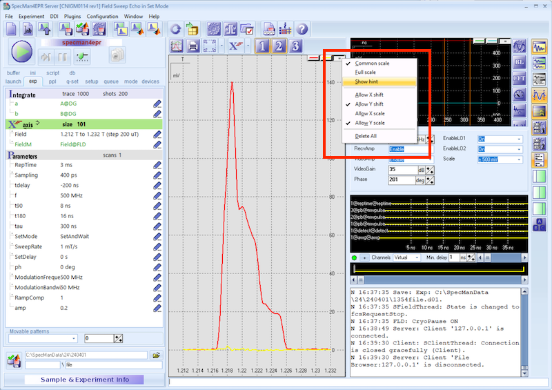
Note down the value of the magnetic field for the maximum echo amplitude. You can enable the cursor by enabling the Hint mode:
Click the right button in the top right corner of the spectrum (see figure below)
From the drop-down menu select Show Hint.
In this particular experiment the field position for the maximum echo amplitude is 1.21865 T.
For nitroxide spin-labels at Q-Band frequencies the separation between the pump and the observe pulse is typically set to 90 MHz, corresponding to 90 MHz / 2.804 = 3.2097 mT.
The field position for the observe pulse is therefore 1.21865 T + 3.2097 mT = 1.221859 T.
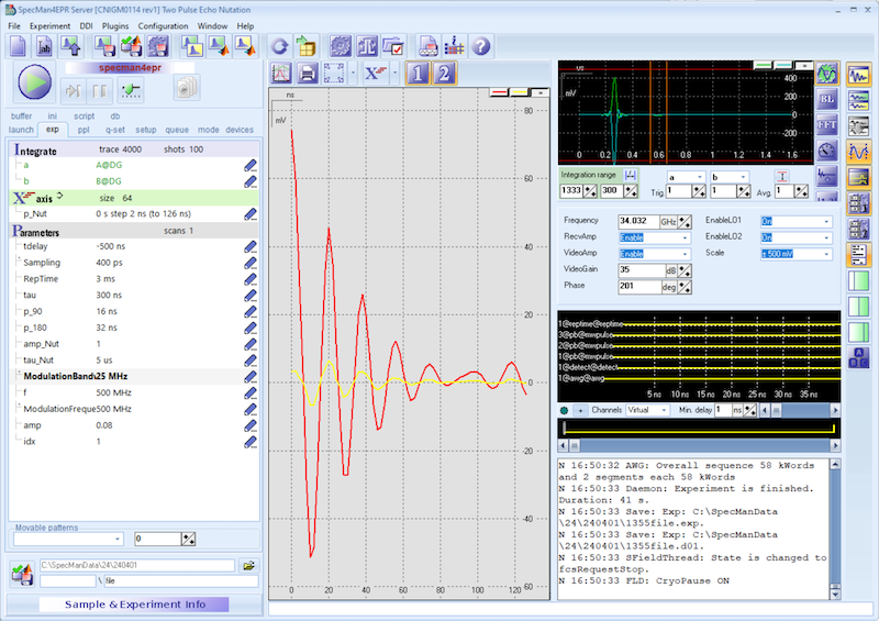
In this section we will provide general instructions on how to run a nutation experiment to determine the optimum length of the inversion pulse.
The nutation is a three pulse experiment. The sequence starts with a nutation pulse followed by a long delay and a two-pulse echo detection sequence. During the experiment the pulse length of the nutation pulse is increased to observe the Rabi oscillation.
To perform the nutation experiment follow these steps:
Start by loading the experiment. From the File menu, select New Experiment. Scroll to the Two Pulse Echo Nutation experiment and click on it to load the experiment.
Make sure the magnetic field is still set to a value corresponding to the maximum echo amplitude (here 1.21865 T).
In the experimental parameter section set the parameter amp_Nut to 1. This is the amplitude for the nutation pulse and we will just use maximum power.
Set pulse length to p_90 = 16 ns and p_180 = 32 ns, set the amplitude for the detection pulses to 0.08 (this is the value that was previously determined).
Hit the tune button and adjust the integration interval in the scope window (vertical orange lines).
To start the experiment, hit the run button.
The result of the experiment is shown in the figure below.
Use the cursor and Hint Mode to determine the pulse length of the inversion pulse. In this case it is 10 ns for an pulse amplitude of 1.
Note
The Bridge12 QLP resonator has a bandwidth of > 400 MHz. Therefore, you don’t have to repeat the nutation experiment at the observe field position.
If you followed the instructions of the previous sections you have all parameters to run a PELDOR/DEER experiment. In this section we show how to setup a PELDOR/DEER experiment. Note, that some parameters such as shots, trace, scans … are set to default values. We recommend to start with these parameters and adjust them later if needed.
First, we need to move the magnetic field to the observe field position:
Open the window to control the field. From the DDI menu select Set Field form, FLD.
Enter the field value for the observe field (here 1.2218 T) and click the Set Field button.
Wait for the field to settle.
In the next step we can setup the PELDOR/DEER experiment:
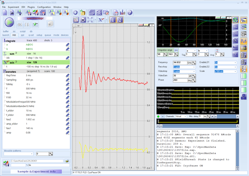
Start by loading the experiment. From the File menu, select New Experiment. Scroll to the 4-Pulse DEER experiment and click on it to load the experiment.
Enter the experimental parameters corresponding to the values determined in the previous section:
Set the pulse length for the observe pulses (t90, t180), the 16 and 32 ns, respectively.
Set the amplitude for the observe pulses (amp) to 0.08. This value was determined in the Optimizing Pulse Parameters section.
Set the value for the maximum dipolar evolution time (tau2) to a value of 1.932 µs.
Set the length of the pump pulse (t_eldor) to 10 ns. This value was determined in the Run a B1 Nutation Experiment section.
Set the amplitude of the pump pulse (amp_eldor) to a value of 1 (maximum power).
Set the frequency of the pump pulse (f_ELDOR) to a value of 590 MHz. The detection is at 500 MHz. Therefore, the overall offset of the pump pulse, with respect to the observe pulse is 90 MHz.
Set the parameter t, the position of the pump pulse to “-100 ns step 16 ns” and the size to 126. Here you should pay attention to the value in the bracket. SpecMan4EPR calculates this value and it should be lower than the value for tau2, the maximum dipolar evolution time.
Enter the number of scans that you would like to run.
Hit the run button to start the experiment.
When you hit the run button, SpecMan4EPR first calculates the entire pulse sequence, including the phase cycle (SpecMan4EPR will step through all variables and you can see this for the different axis). The full pulse sequence is then uploaded to the AWG and the experiment is started. Once a scan is finished and the data is transferred to SpecMan4EPR.
Once the experiment is finished, SpecMan4EPR will automatically save the results. If you want to stop the experiment during the acquisition, you have two choices:
Hit the Run button. This will immediately stop the experiment. In this case the data is not saved automatically.
Hit the Finish button. SpecMan4EPR will finish the current scan before stopping the experiment. The experimental data will be saved.
Setup Overnight experiment
If long signal averaging is required to obtain a sufficient signal to noise ratio, we recommend running the experiment in a queue.
In the experiment panel, select the queue tab (see figure below) top open the queue window.
Click + button (with the green + sign) to add an experiment to queue. This will queue an experiment using the parameters that are currently set in the parameter section.
Click the loop button. By selecting this option, SpecMan4EPR will perform the experiments in the queue (here only ne experiment is added to the queue) and then start over again once all experiments in the queue are finished. The experiment is saved once it finishes.
How to shut down the spectrometer once the experiment is finished
Once all experiments have finished you can shut down the spectrometer.
Shutting down the spectrometer means:
Closing SpecMan4EPR (if desired)
Switching of the microwave amplifier and Q-Band extension
Ramping down the magnetic field to 0 T
Shutting down the spectrometer DOES NOT MEAN:
Switching off the helium compressor
The helium compressor should only be switched off for maintenance or if the spectrometer is not used for a longer time.
Removing the Sample
Follow these steps to remove the sample:
Critically couple the resonator. This will make it easier to find the resonator the next time. Turn the micrometer screw to 0 mm.
Open the resonator tune window (RESONATOR plugin) from the plugins window
Start the tune sweep by clicking the run button (green arrow on bottom left)
You should see a clean tuning picture (see figure below)
To remove the sample:
Make sure you have the blind plug within reach.
Make sure the helium gas pressure inside the cryostat is slightly above atmospheric pressure (> 0.1 bar). Note, the pressure gauge shows a value of 0 bar, when the pressure inside the cryostat is close to atmospheric pressure.
Once the pressure in the cryostat is slightly above atmospheric pressure, it is safe to remove the sample stick. For this loosen the nut and slowly pull out sample stick. While raising the sample stick, observe the tuning picture of the resonator. Once the sample is pulled out of the resonator, the tuning dip of the resonator will disappear (shifted to higher frequency).
Slowly keep raising the sample stick. The sample stick has venting holes at the top and bottom of the G10 section to release helium gas from the cryostat and to purge the sample stick and to prevent air and moisture to enter the sample space.
Once the sample stick is removed from the cryostat secure the sample and either insert a new sample or close the cryostat using the blind plug and tighten the nut. This nut should just be hand-tight. Do not use any tools (e.g. pliers) to close the nut.
Once the cryostat is closed, close the valve to the helium supply.
Start the pump and open the valve to the pump to lower the pressure inside the cryostat to about -0.5 bar. The exact pressure is not important.
Close the valve to the pump.
Ramping Down the Magnetic Field
Once the sample is removed the magnetic field can be ramped down.
Open the window to control the field. From the DDI menu select Set Field form, FLD.
Enter 0 in the field for the magnetic field and hit return.
Under Sweep rate, select the highest sweep rate.
Click the Set Field button to ramp down the magnetic field.
Wait for the field to reach 0 T.
Switching the Spectrometer to Standby Mode
To switch the spectrometer into operate mode:
Select the mode tab from the Experiment Panel.
Click the Standby button. This will disable all synthesizers.
The spectrometer is in standby mode. It is safe to switch off the amplifier and the Q-Band extension.
2 - Quasi-Optics
Quasi-Optical Systems and Components for EPR/DNP Spectroscopy
Quasi optical (QO) systems are used in high-field EPR and DNP systems to control the microwave beam propagation. For example, to separate the incident microwave beam from the reflected beam in a reflection-type EPR bridge. QO is a highly versatile technology to build attenuators, universal polarizers, and beam splitter. If you would like to learn more about it check out our page on Quasi-Optics (QO).
Here you will find the online documentation for some of our QO components. Many QO systems are customer specific. If you have questions about your individual system please contact Bridge12 at support@bridge12.com.
2.1 - Polarizing Transforming Reflector (PTR)
The Bridge12 Polarization Transforming Reflector (PTR) is a universal polarizer. The PTR can convert a linearly polarized microwave beam into a circularly polarized beam, or rotate the E-field vector by any angle.
This is the online documentation of the PTR. For product related information check out the Bridge12 PTR Product Page. The theory and operation of the PTR has been published in:
Chen, Jeson, and Thorsten Maly. “Compact, Tunable Polarization Transforming Reflector for Quasi-Optical Devices Used in Terahertz Science.” Review of Scientific Instruments 93, no. 1 (January 1, 2022): 013102. https://doi.org/10.1063/5.0036292.
If you are using a Bridge12 PTR in your research please consider citing the device in your publication.
2.1.1 - Theory of Operation
The PTR was first described in the literature by Howard et al. operating at a frequency of 28 GHz. Despite its low insertion loss, the PTR has only been used in QO systens for high-field EPR/DNP spectroscopy in some rare instances.
Theory
Wire Grids
Before discussing the PTR in more detail, we will briefly review some fundamental properties of wire grid polarizers.
Free-standing wire grid polarizers made from cylindrical metallic wires either transmit or reflect electromagnetic radiation depending on the orientation (polarization) of the incident E field vector with respect to the grid wire orientation. For cylindrical wires with wire radius \(d\) and wire separation distance \(S\) with \(d \ll S\), the frequency dependent transmission coefficient for an electric field vector oriented parallel to the wire grid can be calculated using the Jones Matrix formalism. The corresponding reflection and transmission matrices are:
This only correct if the grid orientation to be perpendicular to the propagation direction of the beam (\(\theta^{ \prime} = 0^{\circ}\)). However, if the purpose of the grid is to clean up the polarization of the microwave beam, the resulting reflected microwave power should be directed away form the source and not directly reflected back. This can be achieved by orienting the grid at an angle of \(\theta^{\prime} = 45^{\circ}\). In this case determining the reflection and transmission coefficients is less intuitive. This is summarized in the following figure (Figure 1).
Figure 1: Grid orientation for partial beam reflection/transmission
If the grid is oriented perpendicular to the beam propagation direction (\(\theta^{ \prime} = 0^{\circ}\)) the free-standing wire grid needs to be rotated by (\(\theta = 45^{\circ}\)) to transmit 50 % of the power (see Figure 1A). On the other hand, if the grid is oriented at an angle (\(\theta^{ \prime} = 45^{\circ}\)) the wire grid needs to be rotated by (\(\theta = 54.7^{\circ}\)) to transmit 50 % of the power and reflect 50 % of the power (see Figure 1B). For more details check out Paul Goldsmith’s book Quasioptical Systems: Gaussian Beam Quasioptical Propagation and Applications (chapter 8.6.2, page 210).
Figure 2: The free-standing wire grid as a beam splitter
The power transmission and reflection for a variable grid is shown in Figure 2. By rotating the grid and varying the angle \(\theta\) from 0º to 90º the beam can be continuously attenuated. Depending on the quality of the grid this attenuation can reach values of - 30 dB or lower.
Polarization Transforming Reflector (PTR)
The PTR consists of two principle components: 1) A free-standing wire grid and 2) A flat metal reflector. The free-standing wire grid is made from metallic wires having a diameter of d and separated by a distance of S (see figure below). Directly located behind the grid is a flat mirror. A schematic of the PTR is shown in Figure 2 (left).
Figure 2: Bridge12 Polarization Transforming Reflector (PTR). Left: Schematic of the PTR. Right: Dependance of the output polarization from the mirror/grid separation distance. Ev - vertically polarized e-field, Eh - horizontally polarized e-field, Er - right hand circularly polarized e-field, El - left hand circularly polarized e-field.
By changing t, the distance between the flat mirror and the wire grid polarizer of the PTR it is possible to change the polarization state of e.g. a linearly polarized Gaussian incident beam to from linear to circular clockwise and counter-clockwise polarization (Figure 2, right).
How it works
Assuming the gird/mirror pair of the PTR is oriented at angle \(\theta = 45^{\circ}\) with respect to the propagation direction of the incident beam and a grid wire orientation of (\(\theta^{ \prime} = 54.7^{\circ}\)) half of the power of the incident beam will be reflected by the wire grid at point A (see Figure 2, left). The remaining portion of the beam will travel through the grid and be reflected by the flat mirror surface at point B (see Figure 2, left).
Depending upon the distance t between the wire grid and the flat mirror surface, the portion of the beam transmitted by the wire grid will have to travel an additional distance ABC (see Figure 2, left) and will accumulate a phase difference \(\rho\) with respect to the portion of the beam taht is reflected by the wire grid at point A (see Figure 2, left).
For the incoming beam, having a wavelength of \(\lambda \), propagating at an incident angle \(\theta = 45^{\circ}\) and a grid–mirror separation of t, the optical path difference P to travel the additional distance is:
$$ P = AB + BC \\
P = 2t \cos(\theta^{\prime}).
$$
The phase difference \(\rho\) between orthogonal components is given by
$$ \rho = 4 \pi t \cos(\theta^{\prime} \lambda), $$
and the separation distance between orthogonal components \(\Delta\) (beam walk-off, Figure 2 right) is given by
$$ \Delta = 2t \sin(\theta^{\prime}). $$
By changing the distance t, it is possible to change the phase difference between the two beam components and therefore to change the polarization of the e-field of the reflected beam, e.g., from linear to circular or arbitrary linear polarization orthogonal to the propagation axis, with respect to the reflected beam. Choosing the correct distance t, an incident linearly polarized THz beam can therefore be transformed into a beam with a phase difference given by \(\rho\) with respect to the orthogonal polarization. This property enables transformation of, e.g., linear polarization to circular polarization, similar to a quarter-lambda waveplate.
2.1.2 - Installation
The PTR is compatible with the Bridge12 bread-board for quasi-optical instrumentation. The bread-board is based on a 2.5 in. by 2.5 in. grid. It is commonly referred to as a 1 1/2 - 3 - 1 1/2 optic. This means, make sure that there are 2 empty cube positions between two refocusing mirrors.
Installation
To install the PTR:
Slide the dowel pin into the clearance hole of the bread board
Orient the PTR
Lock the PTR position by fastening the 1/2-40 socket head screw
Optimizing the Position
The PTR, as all Bridge12 QO elements only have one degree of freedom (rotation about the dowl pin) to optimize the insertion loss or overall transmission loss of a QO system. To minimize transmission losses:
Loosen the 1/4-20 socket head screw. Do not remove the screw from the bread board
Monitor the transmitted power
Rotate the PTR while maximizing the transmitted power
Note
QO systems can have many individual configurations. In some systems it is easier to monitor the transmitted power, in others it is more convenient to monitor the reflected power. If you are not sure how to optimize the transmission losses in your QO system please contact Bridge12 Technologies, Inc. at support@bridge12.com.
Warning
Do not touch the free-standing wire grid of the PTR. The grid is located at the front of the PTR. The grid is extremely fragile and can be easily destroyed by sharp objects (e.g. screw drivers).
Adapters
The PTR is fully compatible with the Bridge12 QO bread board design. Bridge12 offers adapter plates if you are using a different bread board design. Please contact us at info@bridge12.com for more information.
2.1.3 - Maintenance
The Bridge12 PTR is completely maintenance free. If you experience any problems please contact Bridge12 at support@bridge12.com.
Warning
The free-standing wire grid of the PTR is extremly fragile. Do not use any sharp tools (e.g. blades, screw drivers, etc.) when working around the PTR.
2.1.4 - References
The PTR is not a new device and has been described throughout the scientific literature. Some major references are:
Howard, J., W. A. Peebles, and N. C. Luhmann. “The Use of Polarization Transforming Reflectors for Far-Infrared and Millimeter Waves.” International Journal of Infrared and Millimeter Waves 7 (October 1, 1986): 1591–1603. https://doi.org/10.1007/bf01010760.
Earle, Keith A., Dmitriy S. Tipikin, and Jack H. Freed. “Far-Infrared Electron-Paramagnetic-Resonance Spectrometer Utilizing a Quasioptical Reflection Bridge.” Review of Scientific Instruments 67 (1996): 2502–13.
Amer, N., W. C. Hurlbut, B. J. Norton, Yun-Shik Lee, and T. B. Norris. “Generation of Terahertz Pulses with Arbitrary Elliptical Polarization.” Applied Physics Letters 87, no. 22 (November 28, 2005): 221111. https://doi.org/10.1063/1.2138351.
Chuss, David T., Edward J. Wollack, Ross Henry, Howard Hui, Aaron J. Juarez, Megan Krejny, S. Harvey Moseley, and Giles Novak. “Properties of a Variable-Delay Polarization Modulator.” Applied Optics 51, no. 2 (January 10, 2012): 197. https://doi.org/10.1364/AO.51.000197.
However, when characterizing the PTR developed by Bridge12 Technologies, Inc. we realized that the PTR can also be used as an Universal Polarizer. This properties hasn’t been reported before and was first described in:
Chen, Jeson, and Thorsten Maly. “Compact, Tunable Polarization Transforming Reflector for Quasi-Optical Devices Used in Terahertz Science.” Review of Scientific Instruments 93, no. 1 (January 1, 2022): 013102. https://doi.org/10.1063/5.0036292.
If you are using a PTR manufactured by Bridge12, please consider referencing the above publication.
Initial results were presented at the 2018 ENC Conference as a poster contribution by Jeson Chen.
Poster by Jeson Chen and Thorsten Maly, presented at the 2018 ENC
3 - Accessories
Accessories for EPR/DNP Spectroscopy
3.1 - Active Electric Shims
Online documentation for the Bridge12 active electric shims for elelctromagnets
Welcome to the online documentation of the Bridge12 Active Electric Shims (AES) for electromagnets.
Bridge12 Active Electric Shims (AES)
The Bridge12 AES can be installed in an electromagnet with horizontal field orientation, commonly used in EPR spectroscopy. In total 5 different coils are included to actively control the Z1, Z2, X, and Y gradients. In addition a B0 (Z0) coil is integrated to perform small field adjustments.
Please follow the installation and operation instructions. If you have further questions please contact Bridge12 at support@bridge12.com.
3.1.1 - Installation
Before You Start …
Important
You heard it many times. Before you start assembling the shims we suggest first reading the complete installation instructions to the end and make yourself familiar with the different components. To assemble the shims no further tools are required.
Warning
To install the shims, make sure the magnet is switched off.
What is Included
The Bridge12 AES come by default with the following parts (see figure below):
Bridge12 Active Electric Shims (AES) components
Electrical Shims (right side, qty.: 1)
Electrical Shims (left side, qty.: 1)
Shim spacers (qty.: 4)
Shim supports (qty.: 8)
Adjustment/tightening tool (qty.: 1)
Cables to connect shims to shim interface (qty.: 2)
Shim interface (qty.: 1)
Shim board adapter for Bruker BSMS shim power supply (qty.: 1)
Cable to connect shim interface (7) to Bruker BSMS shim board adapter
Assembling the Shims
Important
Assembling the shims is best done by two people.
The electrical shims are supported between the magnet poles using a total of 8 shim supports and 4 shim spacers (shown in figure below).
Shim Supports (left, right) and Spacer
To assemble the shims:
Place the electrical shims (1 and 2) at the side of the magnet. The board labeled “left” should face the left magnet pole. The board labeled “right” should face the right magnet pole. The labels are located on the back of the boards.
Place the shim spacer between the shim boards
Screw in the shim supports on both side.
The assembly should look similar to the assembly shown in the figure below.
Shims with one set of supports and spacer assembled
Repeat the previous step for all shim supports and spacers.
Alternatively, you can first assemble the shim boards using the supports and the spacers outside the magnet and place the assembled shims between the magnet poles.
Under some circumstances it is not possible to use all 8 shim supports. In this case two supports can be omitted and replaced by two screws as shown in the following image. However, make sure when locking the shims in place that their position is fully secured and that the shims won’t slide down. We don’t recommend removing more than one set of shim supports.
Shims with spacer only
Locking the Shims in Place
Once you have assembled the shims and placed between the magnet pole pieces, you need to lock the shims in place. Each support of the shims has an adjustment screw and a counter nut (see figure below). Before you start turn the counter nut to face the screw as shown in the figure below.
Shim Supports with adjustment screw and counter nut
To hold the shims between the magnet poles, turn the adjustment screws on all sides, until they touch the side of the magnet. Make sure the shims are centered between the pole pieces of the magnet. To turn the screws, especially when the tops of the screws are close to the sides of the magnet use the Adjustment/Tightening tool.
Once the shims are supported between the magnet poles, lock the adjustment screws by turning the counter nut until it touches the shim support. Make sure the nut is not overtightened.
The picture below shows the shims installed in an electromagnet for EPR spectroscopy.
Picture of the installed shims (courtesy of Prof. Song-I Han, UCSB
Connecting the Shims
To use the shims, the following connections have to be made:
Shims to shim interface
Shim interface to shim power supply
Connecting the shims to the shim interface
To connect the shims to the shim interface follow these steps:
Starting with the shims located to the right, connect the ribbon cable marked “RIGHT” to the right shim board.
Connect the same ribbon cable the shim interface.
Repeat the step for the ribbon cable marked “LEFT”.
Connecting the Shims to a Lab Power Supply
The shims can be operated using any benchtop lab power supply. For convenience a multi-channel power supply can be used. Often these power supplies are not bi-polar, in which case you need to swap the leads of the respective channel if you would like to reverse the gradient (e.g. Z1 to -Z1). The power supply can be directly connected to the 15 pin sub-D connector of the shim interface.
Pin# (sub-D)
Shim Connection
Pin# (sub-D)
Shim Connection
1
Z(B)0 (s)
2
Z(B)0 (r)
3
Z1 (s)
4
Z2 (r)
5
Z2 (s)
6
Z2 (r)
7
X (s)
8
X (r)
9
Y (s)
10
Y (r)
15
GND
Shield
GND
(GND - Ground, s - supply, r - return)
Connecting the Shims to a Shim Power Supply
The shims can be operated using a shim power supply e.g. of a NMR spectrometer. The following instructions are specific to a shim power supply used in Bruker NMR consoles (courtesy to Prof. Song-I Han, UCSB).
To connect the shims to a Bruker shim power supply (e.g. BSMS/2) follow this steps:
Connect the shim board adapter to the the shim power supply (see image below, left).
Connect the 15 pin sub-D cable to the shim interface.
Connect the 15 pin sub-D cable to the shim board adapter.
Connecting the shims to the Bruker BSMS/2 shim power supply (images courtesy Prof. Song-I Han, UCSB
Once you have made these connection, the shim can be controlled through the shim power supply.
If you need help at any step of the installation please contact Bridge12 at support@bridge12.com.
3.1.2 - Specifications
The Bridge12 Active Electric Shims (AES) are a 5 channel shim system for electromagnet with a horizontal field. These magnets are typically used in Electron Paramagnetic Resonance (EPR) spectroscopy. The five channels or the shims are: Z0 (or B0), Z1, Z2, X, and Y. Each channel can operate at a current of up to 1.5 A.
Parameter
Value
Number of channels
5
Maximum current/channel
1.5 A
Spacing
53 mm
Warning
Do not exceed a current of (+/-) 1.5 A per channel to avoid permanent damage to the shims.
Shim Interface Pinout
Pin# (sub-D)
Shim Connection
Pin# (sub-D)
Shim Connection
1
Z(B)0 (s)
2
Z(B)0 (r)
3
Z1 (s)
4
Z2 (r)
5
Z2 (s)
6
Z2 (r)
7
X (s)
8
X (r)
9
Y (s)
10
Y (r)
15
GND
Shield
GND
(GND - Ground, s - supply, r - return)
If you need help at any step of the installation please contact Bridge12 at support@bridge12.com.
3.2 - Microwave Power Source
Online documentation for the Bridge12 MPS
We are currently updating the online documentation for the Bridge12 Microwave Power Source (MPS) for ODNP spectroscopy. In the meanwhile, please visit mps.bridge12.com for the previous version.
3.3 - Goniometer
Online documentation for the Bridge12 Goniometer and Control
The goniometer is an attachment for Bridge12 EPR probes, such as the Bridge12 XLP. The accessory is attached to the top of the probe and allows the user to rotate the sample stick around its axis. The goniometer accessory can be fully remote controlled from a terminal window. A Python package is available to allow for complete integration into the spectrometer software.
3.3.1 - Remote Control the Goniometer
How to remote control the goniometer from a computer
The pyB12SMC Python package to remote control the goniometer is available on GitHub (pyB12SMC). To install the Python package follow these steps:
Clone the Python package from the GitHub repository.
Open a terminal window and navigate to the folder to which the Python package was downloaded. For example, if you cloned the repository to C:\Documents\Repositories\pyB12SMC navigate to the folder C:\Documents\Repositories
In the terminal window type the following command and hit the return key:
pip install -e pyB12SMC
Then the Python package will be built and installed locally. Once it is installed you can verify using the pip show command that the package is properly installed:
    B12TManuals % pip show pyB12SMC

    Name: pyB12SMC
    Version: 0.0.1
    Summary: A Python package for interfacing with Stepper Motor Controller (BIGTREETECH SKR MINI E3 V3.0) used in Bridge 12 Technologies products.
    Home-page: http://www.bridge12.com/
    Author: Bridge12 Technologies, Inc
    Author-email: yhuang@bridge12.com
    License:
    Location: /Library/Frameworks/Python.framework/Versions/3.12/lib/python3.12/site-packages
    Editable project location: .../Documents/Repositories/pyB12SMC
    Requires: numpy, pyserial
    Required-by:
The Python package is properly installed and the goniometer can be controlled using the methods in pyB12SMC.
Quickstart - Using the pyB12SMC Python Package
Important
The goniometer rotation is controlled using a stepper motor and the motor is connected to the X axis of the stepper motor controller. Therefore, all commands used to control the goniometer need to reference the X axis..
Once the package is installed open a terminal and start Python. To use the goniometer follow these steps:
Import the Python package
import pyB12SMC
Initialize the class
smc = pyB12SMC.SMC()
Try the following commands:
Go to the home position (X-axis), corresponding to 0º
smc.home('X')
Set the position of the goniometer to 15º
smc.theta('X', 15)
Nothing will happen if the command is repeated since the angle theta is an absolute value. To return to the home position either use one of these two commands:
smc.home('X')
or
smc.theta('X', 0)
To change the behavior from absolute angle to relative angle use the following command:
smc.relative(True)
Now, each time the smc.theta command is issued the goniometer rotates by the given angle. For example:
smc.theta('X', 15)
smc.theta('X', 15)
Will result in a total rotation of 30º.
Sending the following command:
smc.theta('X', -15)
will rotate the goniometer 15º in the opposite direction.
To print an overview of the available methods send the following command:
smc.help()
Troubleshooting
No Serial Communication
If the communication with the controller fails or the device cannot be found, it is possible that the Python package cannot find the device on the COM port. In this case, a COM port can be specified manually. To set the COM port manually (here COM13) send the following command:
smc = pyB12SMC.SMC('COM13')
Method Overview
When starting the Python package an object is created. The methods included in the class are described below.
Important
Valid values for the parameter axis are “X”, “Y”, or “Z” (capital letters)
Method
Returns
Description
move(axis, position)
None
Move axis linearly. Position given in mm.
theta(axis, theta)
None
Move axis rotationally. The angle is given in degrees.
feedrate(axis, feedrate)
None or value (dictionary)
Query the information of federate if no arguments, or set axis feedrate in units/s
position(axis, position)
None or value (dictionary)
Query the information of positions if no arguments, or set axis position in unit
current(axis, current)
None or value (dictionary)
Query the current settings if no arguments, or set axis current in mA
steps_per_unit(axis, step)
None or value
Query the resolutions of all axis if no arguments, or set axis resolution in steps/unit
home(axis)
None
Home all axis if no argument, or home specified axis
set_home(axis)
None
Set current positions as home for all axis if no argument, or set current position as home for an axis
relative(enable)
None or boolean
Query the movement type if no arguments, set movement relative or absolute
save()
None
Save settings to EEPROM
restore()
None
Restore settings from EEPROM
reset()
None
Reset configuration to factory defaults
send_command(command, receive)
None or string
Send command to a device and receive information from a device