Advanced Experiments

• 1: Arraying Parameters
• 2: Calibrating the 90º Pulse Length
• 3: Inversion Recovery Experiments in OVJ
• 4: Creating a Study in OVJ

1 - Arraying Parameters

For many experiments a parameter needs to be varied (e.g. the delay (recovery) time in an inversion-recovery experiment to measure the ¹H longitudinal relaxation time T₁.

In OVJ, this can be done specifying an array of parameters. An array can be either specified through an OVJ GUI or the command line.

It is helpful to first take a look at the pulse sequence to decide, which parameter needs to be arrayed. Either click the ‘Sequence diagram’ button in OVJ or type dps in the OVJ command line. A typical, two pulse experiment is shown in the figure below.

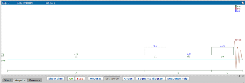
• d1: Repetition time.
• p1: Pulse length of the first pulse. For an inversion recovery experiment, this is the pulse length of the first 180 degree pulse.
• d2: Recovery delay.
• pw: Pulse length of the detection pulse.

Arraying Parameters using the GUI

To use the GUI to define an array of parameters to vary follow these steps:

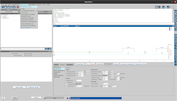
1. In the Acquire Tab click the array button or select Parameter Arrays from the Acquisition menu

   

2. In the window, enter the parameter name to array in the field Param Name. In this example we will vary the parameter d2. The description will be automatically filled in.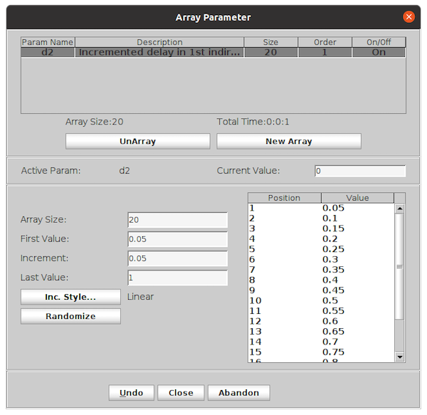

   

3. Enter three of the four parameters (Array Size, First Value, Increment, Last Value). The fourth parameter will be calculated once three values are entered.

   The values of the array is shown in the box to the right. Use the scroll bar see all values of the array.

4. Click the Close button.

   The window will close. The value of the parameter (here d2) will now be displayed as “Array” to indicate an array of values instead of a single value.

Arraying Parameter using the OVJ Command Line

From the OVJ command line, an array can be defined using the array command.

1

array(parameter,number_of_steps,start,step)

For example, to array the parameter d2, starting at 0.05 s, with steps of 0.05 s for a total of 30 points enter the following command:

1

array('d2',30,0.05,0.05)

another possibility to create arrays with arbitrary values is using the syntax $value=val1,val2,…

1

d2=1,4,42

2 - Calibrating the 90º Pulse Length

Calibrating the 90º pulse length is a good example for arraying parameters in OVJ. If you haven’t read the section about how to array parameters in OVJ, we would suggest doing this first before you start to follow this example.

To calibrate the 90 degree pulse length follow these steps:

1. Insert a water sample into the probe.
2. Select the PROTON sequence in OVJ.
3. Set the following parameters in OVJ.
   • Set the sweep width (sw) to a value that the NMR signal (here a single peak from the water sample) is fully within the sweep width of the experiment and some noise is shown left and right to the peak.
   • Set the number of scans (nt) to a value to obtain a clear signal (not too noisy).
   • Set the number of acquired points np to 4096, to acquire 2048 complex points.
4. Array the parameter pw from 0 to about three times the expected pulse length for the 90 degree pulse. In this example we set the array the parameter from 0 to 15 µs with a step size of 0.25 µs.
5. Start the acquisition of the experiment and save the data once the experiment has finished.

The obtained data can be either analyzed in OVJ or dnplab to determine the length of the 90 degree pulse.

Determining the 90 Degree Pulse Length in OVJ

To process the nutation experiment in OVJ follow these steps:

1. After the acquisition select the ‘Process’ tab

   • Select Display and set the display mode for the spectrum to ‘Phased’
   • Select a spectrum that with sufficient signal-to-noise and phase the spectrum. Use a spectrum with a shorter pulse length, don’t use the last spectrum of the nutation experiment. The same phase correction is applied to all spectra in the array.

2. If the sweep width of the spectrum is large, zoom into the region with the peak.

   • Move the mouse cursor to the left of the peak and press the left mouse button. Next, move the mouse cursor to the right of the peak and click the right mouse button. The selected region is shown between the two red lines.
   • Click on the zoom button in the toolbar to the left to zoom into the region defined by the two red lines.

   

3. To show all spectra horizontally aligned, together with their respective pulse length

   • Press the |||| button to show all spectra next to each other

   

   • Next, click # to cycle through the acquisition number or the array parameter

   

4. To show all spectra of the array press the # button in the toolbar

5. The spectrum with the largest peak corresponds to the 90 degree pulse width. In this example the optimum pulse length is 4.75 µs.

   

Determining the 90 Degree Pulse Length in DNPlab

The nutation experiment can also be analyzed in DNPLab. If you haven’t installed DNPLab, this can be easily done using pip:

1

pip3 install dnplab

A typical DNPLab script to determine the 90 degree pulse length is given below:

 1
 2
 3
 4
 5
 6
 7
 8
 9
10
11
12
13
14
15
16
17
18
19
20
21
22
23
24
25
26
27

import dnplab as dnp

data=dnp.load('path/to/folder/PROTON_XY.fid')
data.attrs['experiment_type']='nmr_spectrum'

data=dnp.fourier_transform(data)
data=dnp.autophase(data,dim='t1')

fig,ax=dnp.plt.subplots(1,2)
dnp.plt.sca(ax[0])
dnp.fancy_plot(data)

noise_start_ppm=-1000 #change this according to your spectrum
noise_end_ppm=-500 #change this according to your spectrum
signal_start_ppm=-50 #change this according to your spectrum
signal_end_ppm=50 #change this according to your spectrum

data=dnp.remove_background(data,dim='f2',regions=[(noise_start_ppm,noise_end_ppm)])

data=dnp.integrate(data,regions=[(signal_start_ppm,signal_end_ppm)])

dnp.plt.sca(ax[1])
dnp.fancy_plot(data)
dnp.plt.xlabel('PW (us)')
dnp.plt.ylabel('Signal (a.u.)')

dnp.show()

This processing script first will load the data and does a Fourier transformation of the FID. Next, a DC offset will be removed using the remove_background function. Next, the NMR peak intensity is integrated using the integrate function and the data is plotted using the fancy_plot function.

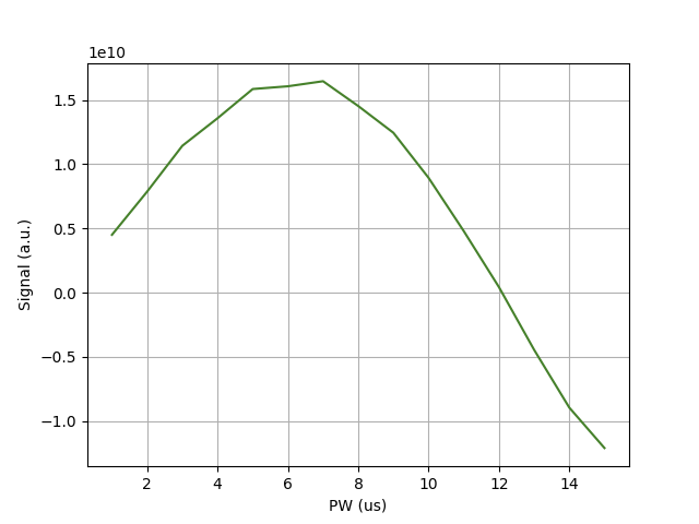
In the example the 90 degree pulse length is about 2.35 µs, and the 180 degree pulse length is about 4.7 µs.

3 - Inversion Recovery Experiments in OVJ

The longitudinal relaxation time T₁ can be determined from an inversion-recovery experiment. This is another good example to demonstrate the arrying capabilities in OVJ. If you haven’t read the section about how to array parameters in OVJ, we would suggest doing this first before you start to follow this example.

The following pre-requisites are assumed:

1. A sample is inserted in the probe.
2. The 90 degree pulse length is know. To determine the correct pulse length please follow the steps outlined in the section Calibrating a 90º Pulse.

Acquire the Inversion Recovery Data

To perform the inversion-recovery experiment follow these steps:

1. Select the PROTON experiment (seqfile='s2pul').

2. Enter the pulse for the 90 degree pulse (pw) and the 180 degree inversion pulse (d1).

3. Enter a value for d1. This is the repetition time of the experiment and it should typically be set to a value of 5 times the T₁ relaxation time of the nucleus. For example, if the relaxation time of the water protons is about 1 s, the value for d1 should be set to 5 s. This ratio can be reduced to speed up the experiment, however, if the repetition time is too short, the measured value for T₁ will be incorrect.

4. For the inversion-recovery experiment we will array the d2 parameter

   1	array('d2',30,0.05,0.05)

5. Press ‘Go’ to start the acquisition or type go and press enter in the OVJ command line.

6. Once the aquisition is finished save the data.

Determining T₁ in OVJ

To determine T₁ in OVJ follow these steps:

1. Select the last spectrum of the array using the ds command. Here, we use spectrum number 15. Alternatively, you can select any spectrum with sufficient signal-to-noise.

   1

   ds(15)

2. Phase the spectrum using the autophase function aph:

   1

   aph

   Once all spectra are phased, you can display all spectra horizontally using the dssh command:

   1

   dssh

   The result should like like the example below

   

   If the spectra look like the data shown in the image proceed to the next step.

3. Select the last spectrum using the ds(15) command.

4. Next, we need to set a threshold for the peak picking algorithm. The threshold is set using the th parameter. In this example, we will set a threshold of 10.

   1

   th=10

   You can also use the horizontal line marker to adjust a threshold. Set the threshold to a value that only one peak is above the threshold.

5. In the next step the peak amplitudes for each spectrum are determined using the dll and fp (find peak) command. Only peaks are considered that are above the threshold value.

   1 2

   dll fp

6. To get the T₁ relaxation time, the t1 OVJ macro can be used. To run the macro, enter t1 in the OVJ command line and press enter.

   1

   t1

7. Display the fitting results using these OVJ command line commands:

   1 2	center expl

   You should see a result similar to the one shown below.

   

   The fit values returned by the t1 macro can be seen in the Process tab under Text output.

   

The t1 macro will create an output file located in the current experiment folder. The path the folder is (N corresponds to the experiment number). The number of the current experiment can be seen in the top left part of the display tab or using the curexp? command in the OVJ command line.

1

~/vnmrsys/expN/analyze.list

Evaluation with dnplab

The inversion-recovery experiment can also be analyzed using DNPLab. First, make sure DNPLab is installed:

1

pip3 install dnplab

A typical processing script is given below:

 1
 2
 3
 4
 5
 6
 7
 8
 9
10
11
12
13
14
15
16
17
18
19
20
21
22
23

import dnplab as dnp

data=dnp.load('path/to/FID/folder')

data=dnp.fourier_transform(data)
data=dnp.autophase(data,dim='t1')

fig,ax=dnp.plt.subplots(1,2)
dnp.plt.sca(ax[0])
dnp.fancy_plot(data)

noise_start_ppm=-1000 #change this according to your spectrum
noise_end_ppm=-500 #change this according to your spectrum
signal_start_ppm=-50 #change this according to your spectrum
signal_end_ppm=50 #change this according to your spectrum

data=dnp.processing.offset.remove_background(data,dim='f2',regions=[(noise_start_ppm,noise_end_ppm)])
data=dnp.processing.integration.integrate(data,regions=[(signal_start_ppm,signal_end_ppm)])

data.attrs['experiment_type']='inversion_recovery'
dnp.plt.sca(ax[1])
dnp.fancy_plot(data)
dnp.show()

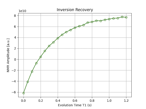
The first subfigure can be used to determine the noise and signal region. The second figure shows the T1 recovery curve. An example for the second figure is shown below.

4 - Creating a Study in OVJ

If the user wants to run a series of experiments a Study should be created in OVJ by the user. The study can be started using the go command and each experiment is automatically saved.

To create a study in OVJ follow these steps:

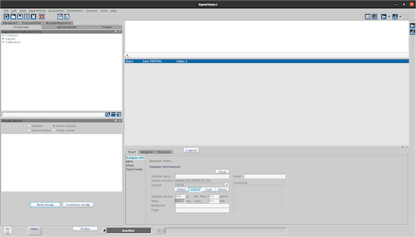
1. Click ‘New study’ in the ‘Study Queue’ tab.

2. Enter a Sample name in the ‘Start’ tab.

   

3. Drag an experiment (e.g. PROTON) from the Experimentor Selector Tree into the Study Queue.

   

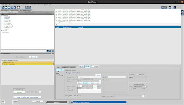
   when the the PROTON_001 sequence is selected (double click) one can adjust all settings for the sequence (Array parameters, change MPS settings, etc..) and when pressing the save button the settings are saved.

   These settings will be the default settings for all experiments in this study. To save the data automatically go to the ‘Acquire’ tab and select ‘Future Actions’.

4. In the ‘When experiment finished’ line enter procsaveplot (select process/plot/save from the dropdown menu) or save to save the data after each ‘go’. Alternatively this can be set with the commandline

   1	wexp='procsaveplot'

5. To start the acquisition of experiments in the study, press the Submit button to start the acquisition.